The tail rotor

The tail rotor operates in a complex flowfield, particularly in low-speed flight, inground effect, sideways flight and in the transition to forward flight. The wake of the main rotor, together with the disturbed air shed from the main rotor hub, rear fuselage and vertical stabilizer, interacts with the tail rotor to create a strongly non-uniform flowfield that can dominate the tail rotor loading and control requirements. The basic

equations for tail rotor forces and moments are similar to those for the main rotor, but a high-fidelity tail rotor model will require a sophisticated formulation for the normal and in-plane components of local induced inflow. Initially, we shall ignore the non-uniform effects described above and derive the tail rotor forces and moments from simple considerations. The interactional effects will be discussed in more detail in Section 3.4.2. The relatively small thrust developed by the tail rotor, compared with the main rotor (between 500 and 1000 lb (2220 and 4440 N) for a Lynx-class helicopter), means that the X and Z components of force are also relatively small and, as a first approximation, we shall ignore these.

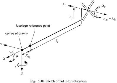
Referring to the tail rotor subsystem in Fig. 3.30, we note that the tail rotor sideforce can be written in the form

Yt = P(atRt)2sra0T(nR2T)(Ft (3.219)

a0TSTj

where ат and Rt are the tail rotor speed and radius, st and a0T the solidity and mean lift curve slope, and Ctt the thrust coefficient given by eqn 3.220:

The scaling factor Ft is introduced here as an empirical fin blockage factor, related to the ratio of fin area Sfn to tail rotor area (Ref. 3.46):

Using the same two-dimensional blade element theory applied to the main rotor thrust derivation, we can write the tail rotor thrust coefficient as

where 0qt and 0* are the effective tail rotor collective and cyclic pitch respectively. Tail rotors are usually designed with a built-in coupling between flap and pitch, the S3 angle, defined by the parameter ^3 = tan S3, hence producing additional pitch inputs when the rotor disc cones and tilts (in MBC parlance). This coupling is designed to reduce transient flapping angles and blade stresses. However, it also results in reduced control sensitivity; the relationship can be written in the form

00T = 0Ot + k-3 вот

0*sT = 01st + hPtsT (3.223)

where 0ot and 0ist are the control-system – and pilot-applied control inputs; the cyclic inputs are usually zero as tail rotors are not normally fitted with a tilting swash plate. Note that the cyclic change is applied at the same azimuth as the flapping, rather than with the 90° phase shift as with swash-plate-applied cyclic on the main rotor; the S3 – applied cyclic is therefore fairly ineffective at reducing disc tilt and is actually likely to give rise to more first harmonic cyclic flapping than would otherwise occur. Again, using the main rotor derivations, particularly the coning relationship in eqn 3.64, we note that the effective collective pitch may be written as

0Ot + k3 ( 872 ) 3 {Hz — 70т)

0*t =——————- ————————————- (3.224)

1 – T (! + HT)

The S3 angle is typically set to -45°, which reduces the tail rotor control effectiveness significantly. The cyclic flap angles can be written in the hub-wind axes form (using the cyclic relationships in eqn 3.64)

(3.225) HT0Ot 2HT (Hzt 7Ot) k3 (3 + 2ht^ ftlswT (3.226)

eicwT —

The tail rotor hub aerodynamic velocities are given by

where the velocities of the tail rotor hub relative to the aircraft centre of gravity have been taken into account, and the factor kiT scales the normal component of main rotor inflow at the tail rotor (at this point no time lag is included, but see later in Chapter 4). The tail rotor uniform inflow is given by the expression

The inflow is determined iteratively in conjunction with the tail rotor thrust coefficient. In the above equations we have assumed that the tail rotor has zero hinge moment, a valid approximation for the rotor forces. For teetering hub blade retention (e. g., in the Bo105), the coning angle at the hub centre can be assumed to be zero and no collective pitch reductions occur.

The tail rotor torque can be derived using the same assumptions as for the main rotor, i. e.,

Qt = – p(QtRt)2nR3T a0T st (—— 2 a0TsT

with induced and profile torque components as defined by

= (Pzr – ^0t)(^CtL) + – OL – (1 + 34)

a0T sT 4a0T

The mean blade drag coefficient is written as

$T = $0T + &2TC T

While the tail rotor torque is quite small, the high rotorspeed results in a significant power consumption, which can be as much as 30% of the main rotor power and is given by the expression

Pt = Qt Qt (3.233)

The tail rotor forces and moments referred to the aircraft centre of gravity are given approximately by the expressions

Xt ~ TtPcT	(3.234)
£ II >7	(3.235)
Zt ~ – TtPisT	(3.236)
Lt ~ hT^T	(3.237)
mT ~ (lT + xcg)ZT – qt	(3.238)
NT = -(lT + xcg)YT	(3.239)

The above expressions undoubtedly reflect a crude approximation to the complex aerodynamic environment in which the tail rotor normally operates, both in low – and high-speed flight. We revisit the complexities of interactional aerodynamics briefly in Section 3.4.2.

3.2.2 Fuselage and empennage