Boundaries with Incoming Disturbances

In many aeroacoustics problems, there are disturbances that enter the computational domain through the outer boundary. For example, in computing the scattering char­acteristics of an object, acoustic waves must be allowed to pass through the boundary of a computational domain in a specified direction and intensity. The scattering phe­nomenon produces scattered waves. These waves are radiated in all directions. They propagate to the far field as outgoing waves through the boundary of the compu­tational domain. In this case, the boundary condition of the computational domain must take on the responsibility of generating the incoming sound and, at the same time, they also serve as radiation boundary conditions for the scattered waves. To handle the dual role, a split-variable method has been developed. The essence of this method is discussed below.

The equations governing the propagation of small-amplitude disturbances are the linearized Euler equations. Both the incoming disturbances and the outgoing scattered waves are solutions of these equations. However, in a scattering problem, incoming disturbances are known or specified, whereas the scattered outgoing waves are unknown. To illustrate the basic concept of the split-variable method, consider a two-dimensional problem with a uniform mean flow velocity u0 in the x direction.

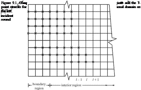It will be assumed that the incoming sound waves enter the computational domain from the left boundary as shown in Figure 9.1. The variables associated with the incoming waves are labeled by a subscript “in” and variables associated with the outgoing scattered waves are labeled by a subscript “out.” In the left boundary region of the computational domain, the total variables are the direct sum of the incoming and outgoing disturbances; i. e.,

In Eq. (9.1) the variables associated with the incoming disturbances are known. They are prescribed by the physical problem. The aim is to compute the outgoing scattered waves. In the boundary region (see Figure 9.1), the outgoing acoustic waves are governed by the radiation boundary condition or Eq. (6.2). That is,

where V(в) = [u0 cos в + (a0 – U sin2 в)1/2] and a0 is the speed of sound.

In the interior region, the small-amplitude disturbances are governed by the linearized Euler equations (see Eq. (5.1)). They are

9 U 9 E 9 F

dt + dx + 9 y

where

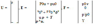(9.3)

Note that the distinction between incoming and outgoing waves is lost once the point of interest is not in the boundary region of the computational mesh.

To compute the numerical solution, Eq. (9.3) is discretized by the 7-point stencil dispersion-relation-preserving (DRP) scheme. These discretized equations are used to determine the full physical variables (p, u, v, p) in the interior region. At the same time Eq. (9.2) is discretized again by the 7-point stencil DRP scheme. These discretized equations are used to calculate the outgoing waves (pout, uout, vout, pout). They are applied only in the boundary region. Before the computation can be implemented, however, one must recognize that once the 7-point stencil DRP scheme is applied to Eq. (9.2), the finite difference stencil in the x direction would extend outside the boundary region into the interior region as shown in Figure 9.1. In the interior region, only the full variables (p, u, v, p) are computed. But (pout, uout, vout, pout) are needed at the extended stencil points to support the computation. To find these quantities, one may use Eq. (9.1). Since the incoming disturbances are known, the outgoing wave variables can be found by subtracting the incoming disturbance variables from the full variables at mesh points near the outer boundary of the interior region.

Now, in computing the full variables (p, u, v, p) in the interior region, one would encounter a similar problem. For mesh points in the three columns closest to the boundary region, the 7-point stencil will extend into the boundary region where only the outgoing disturbances are computed. To find the values of the full variables in the boundary region, one may again use Eq. (9.1) by adding the known incoming disturbances to the computed outgoing waves. In this way, the variables in the entire computational domain can be marched forward in time. It is straightforward to see that the split-variable method essentially converts the boundary region into a source of the incoming disturbances. At the same time, it acts as radiation boundary condition for the outgoing scattered waves.