Flapping Wing and Body Kinematics

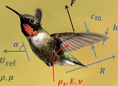
Figure 3.5 illustrates the wing and body movement of a hummingbird, as well as def­initions of some key terms used in this section. The body kinematics is represented by the body angle x (inclination of the body), which is relative to the horizontal plane, and by the stroke plane angle в (indicated by the solid lines), which is defined

(a)

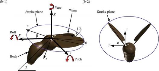
Figure 3.5. (a) Physical variables shown in the case of a hummingbird, (b) Schematic diagram of coordinate systems and wing kinematics, (b-1) The local wing-base-fixed and the global space-fixed coordinate systems. The local wing-base-fixed coordinate system (x, y, z) is fixed on the center of the stroke plane (origin O’ at the wing base) with the д-direction normal to the stroke plane, the у-direction vertical to the body axis, and the z-direction parallel to the stroke plane; (b-2) definition of the positional angle ф, the feathering angle (AoA) a, and elevation angle ф of the flapping wing, the body angle y, and the stroke plane angle ft.

as the plane that includes the wing base and the wingtip’s positions at the maximum and the minimum sweep. The wing-beat kinematics is described by three angles relative to the stroke plane: (i) flapping about the л-axis in the wing-fixed coordinate system described by the positional (flapping) angle ф, (ii) rotation of the wing about

the z-axis described by the elevation (deviation) angle в; and (iii) rotation (feath­ering) of the wing about the у-axis described by the AoA (feathering angle) a. The time history of AoA includes high-frequency modes that are characteristic of some insects [224]. The body angle and the stroke plane angle vary in accordance with the flight speed and flapping wing kinematics of biological flyers [70] [225]. For a general 3D case, a definition of the positional angle, the elevation angle, and the AoA/feathering, all in radians, can be given as follows, for the first four modes:

3

ф() = 0 [Фсп cos (2nn ft) + fsn sin (2nn ft)], (3-1)

n=0

3

в (t) = [ecn cos (2nn ft) + esn sin (2nn ft)], (3-2)

3

a (t) = [acn cos (2nn ft) + asn sin (2nn ft)], (3-3)

Note that n indicates the order of the Fourier series. The Fourier coefficients Фсп, фт, ecn, esn, acn, and asn can be determined from the empirical and measured kinematics data. Wing and body kinematics of biological flyers can be measured by high-speed cameras [226]-[234], laser techniques (a scanning projected line method [235], a reflection beam method [236], a fringe shadow method [237], and a projected comb fringe method [238]), and a combination of high-speed cam­eras and a projected comb-fringe technique with the Landmarks procedure [239]. Advancement in measurement techniques also enables quantification of flapping wing and body kinematics along with the 3D deformation of the flapping wing. Recently, data on the instantaneous wing kinematics involving camber along the span, twisting, and flapping motion have been reported (e. g., a hovering honeybee [240], a hovering hoverfly [241], a free-flying hawkmoth [242], and a bat [243]). Clearly, these efforts have helped establish more complex and useful computa­tional models as well as to develop bio-inspired MAVs. Examples of the kine­matics of a hovering hawkmoth [226] and free-flying hoverflies are plotted in Figure 3.6.

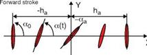
Although 3D effects are important for predicting low Reynolds number flapping wing aerodynamics, 2D experiments and computations do provide valuable insight into the unsteady fluid physics related to flapping wings. Tang, Viieru, and Shyy [244] discussed two hovering modes that are observed in nature: the “water treading” mode [175] and the “normal hovering” mode [217]. The plunging and pitching of the airfoil are described by symmetric, periodic functions:

h (t) = ha sin (2n ft + ф),	(3-4)
a (t) = a0 + aa sin (2n ft),	(3-5)

where ha is the plunging amplitude, f is the plunging frequency, a0 is the initial pitching angle, aa is the pitching amplitude, and ф is the phase difference between plunging and pitching motion. The schematics of the two hovering modes are pre­sented in Figure 3.7. The initial pitching angle for the water treading mode is zero (a0 = 0°), whereas for the normal-flapping/hovering mode a0 = 90°. Figure 3.8 shows

other 2D flapping motions – the pitching and plunging motions – that are more com­monly observed for forward flight. The fluid dynamics based on these kinematics are highlighted in Section 3.5.

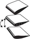
For normal hovering, based on the phase relationship between the translation and rotation of the wing, Dickinson et al. [201] categorized the wing motion into advanced (<p > 90°), synchronized (<p = 90°), and delayed modes (<p < 90°). The

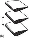
advanced mode (Fig. 3.9a) is the pattern in which the wing rotates before it reverses direction at the end of each stroke. The synchronized mode (Fig. 3.9b) is the pattern

Y
Forward stroke
a
X
Backward stroke
Y
Backward stroke
Y
+aa
‘
X
a
X
a ‘ ‘a (b) “normal” flapping mode
(a) water treading mode
Figure 3.8. Four typical unsteady motions in plung­ing and pitching motion. (a) Combined translational – rotational oscillations, (b) purely translational oscil­lations, (c) purely rotational oscillations, and (d) advancing wave-type deformations. From Rozhdestvensky and Ryzhov [246].
(a)
(c)

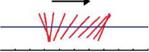
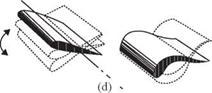
Figure 3.9. Schematics of the three wing rotation patterns: (a) advanced, (b) synchronized, and (c) delayed rotation. As shown in Dickinson et al. [201], the timing of the wing rotation plays an important role in lift generation and, consequently, in maneuvering.

in which the wing rotation synchronizes with its translational motion: its AoA is 90° at the end of each stroke. The delayed mode (Fig. 3.9c) is the pattern in which the wing rotates after it reverses direction at the end of each stroke. Discussion of the effects of the phase relationship on aerodynamic performance is given in Section 3.4.1.