Powerplant and rotor governor

In this section we derive a simplified model for a helicopter’s rotorspeed and associated engine and rotor governor dynamics based on the Helisim powerplant model (Ref. 3.4). The rotorspeed of a turbine-powered helicopter is normally automatically governed to operate over a fairly narrow range with the steady-state relationship given by the equation

Qe = – K3(a – Пі)

where Qe is the turbine engine torque output at the rotor gearbox, Й is the rotorspeed and Q, i is the so-called idling rotorspeed, corresponding to approximately zero engine torque. Equation 3.266 is sometimes described as the droop law of the rotor, the droop constant K3 indicating the reduction in steady-state rotorspeed between autorotation and full power (e. g., in climb or high-speed flight). The rotor control system enforces this droop to prevent any ‘hunting’ that might be experienced should the control law attempt to maintain constant rotorspeed. Rotorspeed control systems typically have two components, one relating the change (or error) in rotorspeed with the fuel flow, af, to the engine, i. e., in transfer function form

-^[Ge(s)] -^ (3.267)

af

the second relating the fuel input to the required engine torque output

a f

—– ► [ He(s)]

The most simple representative form for the fuel control system transfer functions is a first-order lag

a f (s)	Kei 1 + Te1s
Ge(s)	(3.269)

where a bar above a quantity signifies the Laplace transform.

The gain Kei can be selected to give a prescribed rotorspeed droop (e. g., between 5 and 10%) from flight idle fuel flow to maximum contingency fuel flow; we write the ratio of these two values in the form

a fmax a fidle

(3.270)

mi

The time constant re1 will determine how quickly the fuel is pumped to the turbine and, for a fast engine response, needs to be 0(0.1 s).

The engine torque response to the fuel injection can be written as a lead-lag element

1 + re2s 1 + re3s

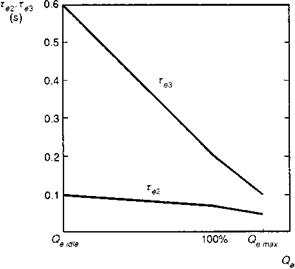
Fig. 3.35 Variation of engine time constants with torque

The gain Ke2 can be set to give, say, 100% Qe at some value of fuel flow rn f (e. g., 75% o)fmax), thus allowing a margin for maximum contingency torque. In the engine model used in Ref 3.4, the time constants in this dynamic element are a function of engine torque. Figure 3.35 illustrates the piecewise relationship showing tighter control at the engine power limit. Linear approximations for the lag and lead constants can be written in the form

%2 — Te2(Qe) ^ T20 + T21 Qe

Te3 — Te3(Qe) ~ T30 + T31 Qe (3.272)

where the time constant coefficients change values at Qe — 100%.

Coupling the two-engine/rotor subsystems gives the transfer function equation

H — Ge (s) He (s) (3.273)

or, in time-domain, differential form

Qe —————- {(Te1 + re3) Qe + Qe + K3 (й — + Te2й)} (3.274)

тЄ1 тЄ3

where

K3 — Ke1 Ke2 —————- Qemax————————————— (3.275)

3 e1 e2 (1 — ttmt) ‘ ‘

and

This second-order, nonlinear differential equation is activated by a change in rotor speed and acceleration. These changes initially come through the dynamics of the rotor/transmission system, assumed here to be represented by a simple equation relating the rotor acceleration (relative to the fuselage, — r) to the applied torque, i. e., the

difference between the applied engine torque and the combination of main rotor Q r and tail rotor torque Qt, referred to the main rotor through the gearing gT, i. e.,

1

^ = r + —(Qe — qr — gTQT) (3.277)

Ir

where Ir is the combined moment of inertia of the rotor hub and blades and rotating transmission through to the free turbine, or clutch if the rotor is disconnected as in autorotation.