PC MATLAB®/SIMULINK®-BASED SIMULATION

Example 6.2

(6.38)

FIGURE 6.13 An unstable aircraft operating in a closed loop. (From Raol, J. R., Girija, G., and Singh, J., Modeling and Parameter Estimation of Dynamic Systems, IEE Control Series, London, 2004.)

q az

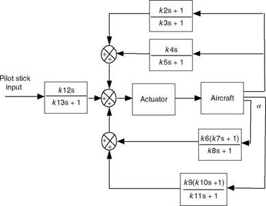
The

The gain values (in the block diagram) used are k2 — 0.125, k3 — 0.212, k4 = 0.519, k5 — 2.0, k6 — 0.519, k7 — 0.13, k8 — 0.3, k9 — 0.0057, k10 — 0.01, k11 — 0.289, k12 — 1.0, k13 — 0.25, and kA — 20.

Solution

The control blocks and plant in Figure 6.13 are realized in SIMULINK. The relevant files are in “ExampSolSW/Example 6.2FS.’’ The simulation responses are obtained by using a doublet input signal with sampling interval of 1 s. Figure 6.14 shows the time histories of the output dynamics of the aircraft with a stabilized controller. It can be observed from the figure that the output responses settle after some transients, hence the controller stabilizes the aircraft. Moreover, the response of the aircraft can be further modified by adjusting gain values judiciously.

Example 6.3

A block diagram representation to generate the aircraft time histories in the presence of turbulence is given in Figure 6.15 [23]. Realize this using MATLAB only. Obtain the responses with and without turbulence. Use the Dryden model for the turbulence and the procedure described here. This model generates moderate turbulence conditions modifying the forward speed, vertical speed, and the pitch rate. The dynamic model of the following form [24,25] is considered:

[ Xu + yukufnJDi/tu

Here, yu and yw are random numbers used for simulating the random nature of the turbulence; tu, tw, ku, and k„ are the time constants:

tu — LujVj; tw — LwjVj; ku — (2s2 tu)/ p; kw — (2ст^)/p (6.45)

Here,

Vj — Ju2 E w2; su — sw; Lu — Lw — 1750 ft (6.46)

Also, L — 1750 ft and the turbulence intensity is s — 3 m/s. This model of turbulence is incorporated into the flight dynamics state equations and a fourth-order Runge-Kutta integration is used to obtain the flight responses of u, w, q, and U and the turbulence response variables xu, xq, xw, and xw. Using the procedure outlined in Refs. [24,25] the turbulence in forward and vertical velocity and pitch rate can be obtained:

qm

Iy

The Dryden model for simulation of turbulence as described above has been used to generate the responses.

Solution

The blocks and their interconnections are realized using MATLAB and the SW is given in “ExampSolSW/Example 6.3Dryden.’’ The aircraft responses with and without turbulence (intensity = 3 m/s) are given in Figure 6.16.

EPILOGUE

The simulation of advanced rotorcraft requires high-fidelity mathematical models. The blade-element theoretic model possesses good fidelity and accuracy for such applications. However, such models with the required complexity would be slow for real-time considerations. Parallel processing would speed up such computations. The blade-element models also possess flexibility. In Ref. [26] an advanced rotorcraft flight simulation model is developed and it is specially suited to implementation on a parallel computer. In Ref. [27] the concept of using flight-recorded data for pilot training via RTS playback of flight maneuvers is developed. It also details the requirements for simulation-based flight reconstruction. A robust KF is used as a

state-estimator flight simulator driver. The methodology is validated for UH-60 helicopter nonlinear simulation. A procedure that combined the three steps is presented in Ref. [28]: identification of derivatives in linear/nonlinear models, comparison of the results to the original database, and update of the database if necessary. Further development of the nonlinear model can be found in Ref. [29]. In Ref. [30] the complete development of a 3DOF motion-based flight simulator is described. Nowadays well-validated flight simulation/control analysis SW packages are available [3,15,31].

EXERCISES

6.1 The aero database is given in the form of lookup tables (Section 6.2.1). Explain the theory of the Table lookup.

6.2 A system of equations with a wide variety of time constants, for the same dynamic system, is known as a stiff system of equations. What problem would it pose for the solution of these equations by the Runge-Kutta (RK) method?

6.3 The following are nonlinear state-space equations: x(f) = u(t)). Linearize

this system of equations using Taylor-series expansion.

6.4 Obtain the TF, Bode diagram, and step response of the elevator actuator model of Table 6.1. Also, use the booster dynamics: s2+52 293+3283 3 in conjunction with the actuator TF and obtain the composite TF model, its Bode diagram, and step response.

6.5 Obtain the Bode diagrams for the inner ears’ models of Equations 6.2 and 6.3.

6.6 Represent the basic elements’ operations of an INS in the form of a block diagram.

6.7 Take appropriate SI units and verify the formula dimensionally/units wise:

Qo = CdiAo^f.

6.8 In an actual aircraft what is the mechanism for trimming? In which way would a trim device help the pilot?

6.9 What is trimming IFS with respect to the EOMs/flight dynamics? Explain with reference to the state-space Equation 2.10.

6.10 In computer simulation of the dynamic equation of an aircraft or other systems, we may have to slow down or obtain a fast solution. For this, scaling is required to be done: t = at, where t is the computer time and “a” is the scale. Explain the significance of this with an example of a second-order system.