Appendix 3A Frames of Reference and Coordinate Transformations

3A.1 The inertial motion of the aircraft

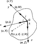
In this section we shall derive the equations of translational and rotational motion of a helicopter assumed to be a rigid body, referred to an axes system fixed at the centre of

Fig. 3A.1 The fuselage-fixed reference axes system

mass of the aircraft (assumed to be fixed in the aircraft). The axes, illustrated in Fig. 3A.1, move with time-varying velocity components u, v, w and p, q, r, under the action of applied forces X, Y, Z and L, M, N.

The evolutionary equations of motion can be derived by equating the rates of change of the linear and angular momentum to the applied forces and moments. Assum­ing constant mass, the equations are conveniently constructed by selecting an arbitrary material point, P, inside the fuselage and by deriving the expression for the absolute acceleration of this point. The acceleration can then be integrated over the fuselage volume to derive the effective change in angular momentum and hence the total inertia force. A similar process leads to the angular acceleration and corresponding inertial moment. The centre of the moving axes is located at the helicopter’s centre of mass, G. As the helicopter translates and rotates, the axes therefore remain fixed to material points in the fuselage. This is an approximation since the flapping and lagging motion of the rotor cause its centre of mass to shift and wobble about some mean position, but we shall neglect this effect, the mass of the blades being typically <5% of the total mass of the helicopter. In Fig 3A.1, i, j, k are unit vectors along the x, y andz axes respectively.

We can derive the expression for the absolute acceleration of the material point P by summing together the acceleration of P relative to G and the acceleration of G relative to fixed earth. The process is initiated by considering the position vector of the point P relative to G, namely

r p/g = x i + yj + zk (3A.1)

The velocity can then be written as

v p/g = Г p/g = (x i + yj + zk) + (xi + yj + zk) (3A.2)

Since the reference axes system is moving, the unit vectors change direction and therefore have time derivatives; these can be derived by considering small changes in the angles 80, about each axis. Hence

8i = j80z — k80y

di d9z d0y

d =i = j dT – k IT =rj – q k

Defining the angular velocity vector as

Mg = pi + q j + r k (3A.5)

we note from eqn 3A.4 that the unit vector derivatives can be written as the vector product

i = Mg л i

with similar forms about the j and k axes.

Since the fuselage is assumed to be rigid, the distance of the material point P from the centre of mass is fixed and the velocity of P relative to G can be written as

vp/g = Mg л rp (3A.7)

or in expanded form as

vp/g = (qz – ry)i + (rx – pz)j + (py – qx)k = Up/gi + Vp/gj + Wp/gk (3A.8)

Similarly, the acceleration of P relative to G can be written as

a p/g = v p/g = (up/gi + vp/gj + wp/gk) + (up/gi + vp/gj + wp/gkk)

= ap/grel + Mg л vp (3A.9)

or, in expanded form, as

ap/g = (up/g – rvp/g + qwp/g)i +(v p/g – pwp/g + rup/g)j

+ (wp/g – qup/g + pvp/g)k (3A.10)

Writing the inertial velocity (relative to fixed earth) of the aircraft centre of mass, G, in component form as

Vg = ui + vj + w k (3A.11)

we can write the velocity of P relative to the earth reference as

vp = (u – ry + qz)i + (v – pz + rx)j + (w – qx + py)k (3A.12)

Similarly, the acceleration of P takes the form

ap = aprel + Mg л Vp (3A.13)

or

with components

ax = u – rv + qw – x(q2 + r2) + y(pq – r) + z(pr + q) (3A.15)

ay = v – pw + ru – y(p2 + r2) + z(qr – p) + x(pq + r) (3A.16)

az = w – qu + pv – z(p2 + r2) + x(pr – q) + y(qr + p) (3A.17)

These are the components of acceleration of a point distance x, y, z from the centre of mass when the velocity components of the axes are given by u(t), v(t), w(t) and p(t), q(t), r(t).

We now assume that the sum of the external forces acting on the aircraft can be written in component form acting at the centre of mass, i. e.,

Fg = X i + Yj + Z k (3A.18)

If the material point, P, consists of an element of mass dm, then the total inertia force acting on the fuselage is the sum of all elemental forces; the equations of motion thus take the component forms

Ma = j dm

body

The translational equations of motion of the aircraft are therefore given by the relatively simple equations

X = Ma(u – rv + qw)

Y = Ma(v – pw + ru)

Z = Ma(w – qu + pv) (3A.24)

Thus, in addition to the linear acceleration of the centre of mass, the inertial loading is composed of the centrifugal terms when the aircraft is manoeuvring with rotational
motion. For the rotational motion itself, the external moment vector about the centre of mass can be written in the form

Mg = L i + Mj + N к

Considering the component of rolling motion about the fuselage x-axis, we have

L = j (yaz — zay) dm

body

and substituting for ay and az we obtain
L = p (y2 + z2) dm —	qr / (z2 — y2) dm + (r2	— q2) 1 yz dm
J body	J body	J body
— (pq + r) 1 xz dm + (pr — q) 1 xy dm	(3A.28)
body	body
Defining the moments and product (Ixz) of inertia as
x-axis:	hx = f (y2 + z2) dm	(3A.29)
	J body
y-axis:	Iyy = 1 (x2 + z2) dm	(3A.30)
	J body
z-axis :	hz = f (x2 + y2) dm	(3A.31)
	J body
xz	-axes: Ixz = 1 xz dm	(3A.32)

body

we note that the external moments can finally be equated to the inertial moments in the form

The product of inertia, Ixz, is retained because of the characteristic asymmetry of the fuselage shape in the xz plane, giving typical values of Ixz comparable to Ixx.

3A.2 The orientation problem – angular coordinates of the aircraft

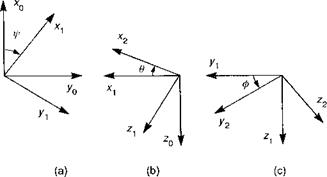
The helicopter fuselage can take up a new position by rotations about three independent directions. The new position is not unique, since the finite orientations are not vector quantities, and the rotation sequence is not permutable. The standard sequence used in flight dynamics is yaw, ф, pitch, 9, and roll, ф, as illustrated in Fig. 3A.2. We can consider the initial position as a quite general one and the fuselage is first rotated about the z-axis (unit vector k0) through the angle ф (yaw). The unit vectors in the rotated frame can be related to those in the original frame by the transformation Ф, i. e.,

i1		cosф	sinф	0	io "
j1	=	—sinф	cosф	0	jo	or {b} = W{a}	(3A.34)
k)_		0	0	1_	_ko_

Next, the fuselage is rotated about the new y-axis (unit vector j1) through the (pitch) angle 9, i. e.,

i2		cos 9	0	— sin 9	i1
j1	=	0	1	0	j1	or {c} = 0{b}	(3A.35)
k1		sin 9	0	cos 9	_ko_

Finally, the rotation is about the x-axis (roll), through the angle ф, i. e.,

i2		1	0	0	i2
j2 k2	=	0 0	cos ф — sin ф	sin ф cos ф	1——– 1_____	or {d} = Ф{с}	(3A.36)

Any vector, d, in the new axes system can therefore be related to the components in the original system by the relationship

{d} = Ф0Ф {a} = Г {a} (3A.37)

Fig. 3A.2 The fuselage Euler angles: (a) yaw; (b) pitch; (c) roll

Since all the transformation matrices are themselves orthogonal, i. e.,

фт = ф-1 , etc. (3A.38)

the product is also orthogonal, hence

rT = Г-1 (3A.39)

where

cos 9 cos f	cos 9 sin f	— sin 9
sin ф sin 9 cos f—	sin ф sin 9 sin f+	sin ф cos 9
cos ф sin f	cos фcos f		(3A.40)
cos ф sin 9 cos f+	cos ф sin 9 sin f —	cos ф cos 9
sin ф sin f	sin ф cos f

Of particular interest is the relationship between the time rate of change of the orien­tation angles and the fuselage angular velocities in the body axes system, i. e.,

Mg = ph + qji + r k2

= f ko + 9ji + ф І2 (3A.41)

Using eqns 3A.34-3A.36, we can derive

p = ф — f sin 9 q = 9 cos ф + f sin ф cos 9

r = —9 sin ф + f cos ф cos 9 (3A.42)

3A.3 Components of gravitational acceleration along the aircraft axes

The relationships derived in Appendix Section 3A.2 are particularly important in flight dynamics as the gravitational components appear in the equations of motion in terms of the so-called Euler angles, 9, ф, f, while the aerodynamic forces are referenced directly to the fuselage angular motion. We assume for helicopter flight dynamics that the gravitational force always acts in the vertical sense and the components in the fuselage-fixed axes are therefore easily obtained with reference to the transforma­tion matrix given in eqn 3A.40. The gravitational acceleration components along the fuselage x, y and z axes can therefore be written in terms of the Euler roll and pitch angles as

axg = ~g sin 9 ayg = g cos 9 sin ф aZg = g cos 9 cos ф

3A.4 The rotor system – kinematics of a blade element

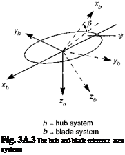
The components of velocity and acceleration of a blade element relative to the air through which it is travelling, and the inertial axes system, are important for calculating the blade dynamics and loads. When the hub is fixed, the only accelerations experienced by a flapping blade are due to the centrifugal force and out-of-plane motion. When the hub is free to translate and rotate, then the velocities and accelerations of the hub contribute to the accelerations at a blade element. We begin with an analysis of the transformation between vectors in the non-rotating hub reference system and vectors in the blade axes system.

Figure 3A.3 illustrates the hub reference axes, with the x and y directions oriented parallel to the fuselage axes centred at the centre of mass. The z direction is directed downwards along the rotor shaft, which, in turn, is tilted forward relative to the fuselage z-axis by an angle ys. The blade referenced axes system has the positive x direction along the blade quarter chord line. The zero azimuth position is conventionally at the rear of the disc as shown in the figure, with the positive rotation anticlockwise when viewed from above, i. e., in the negative sense about the z-axis. Positive flapping is upwards. The positive y and z directions are such that the blade and hub systems align when the flapping is zero and the azimuth angle is 180°.

We shall derive the relationship between components in the rotating and non­rotating systems by considering the unit vectors. The orientation sequence is first azimuth, then flap. Translational and angular velocities and accelerations in the hub system can be related to the blade system by the transformation

ih		— cos ф	— sin ф	0	cos в	0	sin в	ib
jh	=	sin ф	— cos ф	0	0	1	0	jb
_ kh _		0	0	1	— sin в	0	cos в	_ kb _

(3A.44)

or, in expanded form

ih		— cos ф cos в	— sin ф	— cos ф sin в	ib
jh	=	sin ф cos в	— cos ф	sin ф sin в	jb
kh		— sin в	0	cos в	kb

The hub velocity components in the hub reference system are related to the velocities of the centre of mass, u, v and w through the transformation

uh		cos Ys	0	sin Ys		u — qhg
vh	—	0	1	0		v + phR + rxcg	(3A.46)
wh		_- sin Ys	0	cos Ys		_ w — qxcg

where ys is the forward tilt of the rotor shaft, and h r and xcg are the distances of the rotor hub relative to the aircraft centre of mass, along the negative z direction and forward x direction (fuselage reference axes) respectively.

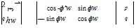
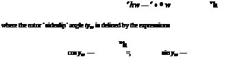
It is more convenient, in the derivation of rotor kinematics and loads, to refer to a non-rotating hub axes system which is aligned with the resultant velocity in the plane of the rotor disc; we refer to this system as the hub-wind system, with subscript hw. The translational velocity vector of the hub can therefore be written with just two components, i. e.,

vhw — uhw ihw + whw khw

The angular velocity of the hub takes the form

&hw — phw ihw + qhw jhw + rhw khw

The hub-wind velocities are given by the relationships

/ 2 2 1/2

uhw — uh cos фw + vh sin фw — [uh + vh)

vhw — 0

whw — wh

lul + v2

lul + v2

(3A.50)

We now write the angular velocity components transformed to the rotating system as

(3A.53)

station rb, in the blade axes system, may be written as

ub = uhw cos f whw p

vb = – uhw sin f – rb (fi – rhw + P&x)

wb = – uhwв cos f + whw + rb {<j)y – p) (3A.54)

Similarly, the blade accelerations can be derived, but in this case the number of terms increases considerably. The dominant effects are due to the acceleration of the blade element relative to the hub, with the centrifugal and Coriolis inertia forces giving values typically greater than 500 g at the blade tip. Blade normal accelerations are an order of magnitude smaller than this, but are still an order of magnitude greater than the mean accelerations of the aircraft centre of mass and rotor hub. We shall therefore neglect the translational accelerations of the hub and many of the smaller nonlinear terms due to products of hub and blade velocities. The approximate acceleration components at the blade station are then given by the expressions

axb = rb(- (fi rhw) + 2p^y 2 (fi rhw) P^x’j

ayb = rb (-(fi – rhw) – P(qhw sin f – phw cos f) + rhw P^y)

azb = rb(^2Qo)x + (qhw cos f + phw sin f – rhw&x – (fi – rhw)2p – pj

(3A.55)

The underscored components are the primary effects due to centrifugal and Coriolis forces and the angular accelerations of the hub, although the latter are also quite small in most cases. For practical purposes, we can usually make the additional assumption that the rotorspeed is much higher than the fuselage yaw rate, so that

(fi – rhw) ~ fi (3A.56)