PML in Three Dimensions

In three dimensions, the linearized Euler equations may be written in a matrix form

as

d u 9 u „ 9 u

+ A + В

dt dx dy

where

p		M	1	0	0	0		0	0	1	0	0		0	0	0	1	0
u		0	M	0	0	1		0	0	0	0	0		0	0	0	0	0
v	, a =	0	0	M	0	0	, В =	0	0	0	0	1	, c =	0	0	0	0	0
w		0	0	0	M	0		0	0	0	0	0		0	0	0	0	1
p_		0	1	0	0	M		0	0	1	0	0		0	0	0	1	0

A straightforward application of the method of Section 9.5.1 yields the following PML equations:

Figure 9.13. PML for circular ducted computational domain.

where

u + (ay + az )ql + ayazq2 u + (az + ax )ql + azaxq2

U + (ax + ay )ql + axayQ2

(ax + ay + az)U + (ayaz + azax + axay )4l + axayaz02-

The auxiliary variables ql and q2 are given by

Notice that the absorption coefficients ax, a and az are arbitrary functions of x, y, and z, respectively. Again, as in the two-dimensional case, the auxiliary variables, q1 and q2 need to be computed only in the PML regions.

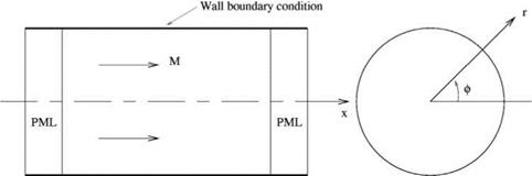
The PML absorbing boundary condition is especially useful in a ducted envi­ronment. It is very effective for simulating a long-duct termination. Figure 9.13 shows a computational domain inside a circular duct with rigid walls. In cylindrical coordinates, (x, r, ф), the linearized Euler equations may be written as

where

	p					M	1	0	0	0		0	0	1	0	0
	u					0	M	0	0	1		0	0	0	0	0
U =	v	,		a	=	0	0	M	0	0	,	В=	0	0	0	0	1
	w					0	0	0	M	0		0	0	0	0	0
	p _					0	1	0	0	M		0	0	1	0	0
	‘ 0	0	0	1	0 ‘			‘ 0	0	1 0	0
	0	0	0	0	0			0	0	о о	0
C=	0	0	0	0	0	, d	=	0	0	О О	0
	0	0	0	0	1			0	0	О О	0
	0	0	0	1	0			0	0	1 0	0

The corresponding PML equation is

where

In applying PML to a ducted domain, the wall boundary condition for the PML is the same as that for the Euler domain. For instance, for the rigid wall circular duct problem of Figure 9.13, the same rigid wall boundary condition, namely, v = 0, at r = D/2 is to be used in the PML regions.

In implementing PML, the damping coefficients, say, ctx(x), cty(y), are often taken as smooth functions. A good practice is to set these functions equal to zero at the interface with the Euler domain. It is also a good practice to let ctx(x) increase smoothly to a constant level in the main part of the PML. At the termination of the PML, the computed variables are usually exponentially small so that reflection is not a concern. However, it is a good practice to impose a standard radiation boundary condition that is of minimal cost to the computation.