The general trim problem

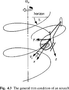
The elementary analysis outlined above illustrates the primary mechanisms of trim and provides some insight into the required pilot trim strategy, but is too crude to be of any real practical use. The most general trim condition resembles a spin mode illustrated in Fig. 4.3. The spin axis is always directed vertically in the trim, thus ensuring that the rates of change of the Euler angles 9 and ф are both zero, and hence the gravitational force components are constant. The aircraft can be climbing or descending and flying out of lateral balance with sideslip. The general condition requires that the rate of change of magnitude of the velocity vector is identically zero. Considering eqns 3.1-3.6 from Chapter 3, we see that the trim forms reduce to

where the reader is reminded that the subscript e refers to the equilibrium condition. For the case where the turn rate is zero, the applied aerodynamic loads, Xe, Ye and Ze, balance the gravitational force components and the applied moments Le, Me and Ne are zero. For a non-zero turn rate, the non-zero inertial forces and moments (centrifugal, Coriolis, gyroscopic) are included in the trim balance. For our first-order approximation, we assume that the applied forces and moments are functions of the translational velocities (u, v, w), the angular velocities (p, q, r) and the rotor controls ($0, в1s, $ic, $0T). The Euler angles are given by the relationship between the body axis angular rates and the rate of change of Euler angle Ф, the turn rate about the vertical axis, given in eqn 3A.42, i. e.,

Pe = -‘І/e sin &e (4.29)

Qe = Фe sin Фє cos ®e (4.30)

Re = vpe cos Фє cos &e (4.31)

The combination of 13 unknowns and 9 equations means that to define a unique solution, four of the variables may be viewed as arbitrary and must be prescribed. The prescription is itself somewhat arbitrary, although particular groupings have become more popular and convenient than others. We shall concern ourselves with the classic case where the four prescribed trim states are defined as in Fig. 4.3, i. e.,

In Appendix 4C, the relationships between the prescribed trim conditions and the body axis aerodynamic velocities are derived. In particular, an expression for the track angle between the projection of the fuselage x-axis and the projection of the flight velocity
vector, both onto the horizontal plane, is given by the numerical solution of a nonlinear equation. Since the trim eqns 4.23-4.28 are nonlinear, and are usually solved iteratively, initial values of some of the unknown flight states need to be estimated before they are calculated. In the following sequence of calculations, initial values are estimated for the Euler pitch and roll angles 0e and Фє, the rotorspeed Q r, the main and tail rotor uniform downwash components Xo and Лот and the main rotor lateral flapping angle ви.

The solution of the trim problem can be found by using a number of different techniques, many of which are available as closed software packages, that find the minimum of a set of nonlinear equations within defined constraints. The sequential process outlined below and summarized in Fig. 4.4 is recognized as rather inefficient in view of the multiple iteration loops – one for pitch, one for roll, one for rotorspeed and one for each of the downwash components – but it does enable us to describe a sequence of partial trims, provides some physical insight into the trim process and can assist in identifying ‘trim locks’, or regions of the flight envelope where it becomes difficult or even impossible to find a trim solution. The process is expanded as a sequence in Fig. 4.5. The first stage is the computation of the aerodynamic velocities, enabling the fuselage forces and moments to be calculated, using the initial estimates of aerodynamic incidence angles. The three iteration loops can then be cycled.