Impedance Boundary Condition in the Presence of a Subsonic Mean Flow

In jet engines, there is invariably a mean flow adjacent to the acoustic liners. Tradi­tionally, impedance boundary condition in the presence of a mean flow is formulated with the assumption of the existence of a very thin zero-velocity fluid layer at the sur­face of the acoustic liner (see Figure 10.6). At the interface of the zero-velocity fluid layer and the mean flow, the condition of continuity of particle displacement is used. In dimensionless variables the frequency-domain impedance boundary condition on liner surface S0(x, y, z) = 0, derived by Myers (1980), is

rnvnZ + (-іш + U-V) p = pn-(n-V )U,

where U is the mean flow velocity on the liner surface, n is the unit outward pointing normal of S0; that is, n = VS0/|VS0|. vn is the velocity normal to S0 with positive pointing into the liner. If the three-parameter model for Z is used, the time-domain impedance boundary condition is

For the special case for which S0 is a plane as shown in Figure 10.6, the frequency – domain impedance boundary condition, after simplification, may be written as

— іш + M—^ = – rnZvn. (10.13)

9 x

In an extensive numerical study of the normal modes of a duct with acoustic lin­ers, Tester (1973) found that boundary condition (10.13) led to an unstable solution. The unstable solution is of the Kelvin-Helmholtz-type instability arising from the vortex sheet interface between the mean flow and the zero-velocity fluid layer. In standard duct acoustics analysis using the frequency-domain approach, this instabil­ity is either not mentioned or totally bypassed and ignored. Now, it is easy to show that the use of boundary condition (10.13) always gives rise to an unstable solution.

The linearized momentum and energy equations governing the sound field superimposed on a uniform mean flow of Mach number M in the x direction (see Figure 10.6) are as follows:

where O = ю — Ma, к = (a2 + в2)1/2, and O = O/к. The branch cuts of the square root function (O2 -1)1/2 are the same as those stipulated in Figure 10.4 with O replacing о and к set equal to 1.

(O2 — 1) 2

Substitution of solution (10.16) into the Fourier-Laplace transforms of boundary condition (10.13) yields the following dispersion relation:

1 (O2 — 1) 2

Now, let the left side of Eq. (10.17) be denoted by f (O) as follows:

Figure 10.7 shows the map of the upper-half O plane in the f plane (shaded region) for X > 0. Since a can be positive or negative, there will always be values of a for which the point representing the right side of Eq. (10.17) lies in the shaded region of the f plane. Therefore, there will always be an unstable solution. If X is negative, a similar mapping procedure will show that there is always an unstable solution.

The existence of a Kelvin-Helmholtz-type instability renders the boundary value problem ill-posed for the time-domain solution. The instability is, however, non­physical. Its origin is in the postulate of a vortex sheet discontinuity right next to the impedance boundary. In reality, no such vortex sheet exists in the flow. For time-domain problems, the instability is weak. It can be effectively suppressed by the addition of artificial selective damping near and at the surface of the acoustic liner. With the weak instability suppressed, boundary condition (10.13) has yielded solutions that are in agreement with frequency-domain calculations.

Figure 10.7. Map of the upper-half a> plane in the f plane (X > 0): (a) a> plane, (b) f plane.

10.1 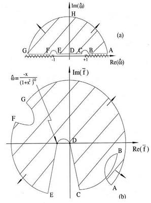Numerical Implementation

On incorporating the effect of convection (see Eq. (10.13)) the time-domain impedance boundary condition (10.4) or the Myers (1980) boundary condition

becomes

^+m ^ = я Ті – X v + X dt + dx dt -1 " + 1

The numerical implementation of this boundary condition will considered.

Let a large acoustically treated panel be lying on the x-z plane as shown in Figure 10.3. It will be assumed that there is a uniform flow adjacent to the panel. The governing equations of the acoustic field are the linearized Euler equations. In dimensionless form, these equations are

Now consider a computational domain as shown in Figure 10.8. y = 0 is the surface of the acoustically treated panel. Eqs. (10.20) to (10.24) apply to every grid point on the mesh. This includes the boundary points at y = 0 or m = 0, where m is the mesh index in the y direction. However, boundary condition (10.19) also applies to the boundary mesh point at y = 0 or m = 0. This means that there are more equations than unknowns. To resolve this problem of an overdetermined system, a row of ghost values of pressure, pe _1 k is introduced at m = -1, the ghost point. Here, subscripts I and к are the mesh indices in the x and z directions, respectively. Including the ghost values, the number of equations and unknowns are exactly equal. Since the ghost values are not governed by a time-dependent equation, it is necessary to combine boundary condition and equations of motion to reduce one of the equations effectively to a form without a time derivative. This form of the boundary condition is then used to determine the ghost values.

To facilitate the implementation of the time-domain impedance boundary con­dition (10.19), an auxiliary variable q(x, z, t), defined at y = 0 by

is introduced. q is only defined on the acoustic liner surface; i. e., y = 0. Note: vn = – v for the flow configuration of Figure 10.3. Boundary condition (10.19) may be rewritten, after eliminating дp/дt by Eq. (10.24), as follows:

^ = q _ m^. (10.27)

dy dx

Eq. (10.27) does not contain time derivative. It is in a suitable form for use to determine the ghost value pl -1k.

The discretized form of Eq. (10.27) using the backward difference stencil of Figure 10.8 is

where Ax and Ay are the mesh sizes. On solving for the ghost value, it is straightfor­ward to find

On choosing the ghost value by Eq. (10.28), the governing Eq. (10.27) or its progenitor Eq. (10.22) is automatically satisfied. To compute the entire sound field, the values of p, u, w, and p at every mesh point (l, m, k) are calculated by Eqs. (10.20), (10.21), (10.23), and (10.24). For velocity component v at all mesh points, except those on the acoustically treated panel surface, i. e., m = 0, the value is updated by means of Eq. (10.22). For mesh points at m = 0, vl,0,k are computed by Eq. (10.25). The auxiliary variable q is to be calculated by Eq. (10.26). In discretizing the spatial derivatives in y for mesh points in rows m = 0,1,2, the backward difference stencils shown in Figure 10.8 are to be used. Finally, artificial selective damping must be added to each time-dependent equation to suppress the weak instability of the impedance model.