Stability of the Three-Parameter Time-Domain Impedance Boundary Condition

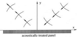
The time-domain impedance boundary condition (10.4) may not be used unless it leads to a stable solution. To show that an acoustic problem with (10.4) as boundary condition is computationally stable, consider a plane acoustic liner adjacent to a sound field as shown in Figure 10.3. For simplicity, let the surface of the liner be the x-z plane. In terms of dimensionless variables with L (a typical length of the problem) as the length scale, a0 (the sound speed) as the velocity scale, L/a0 as

Figure 10.3. Sound field adjacent to an acoustically treated panel.

the time scale, p0 (the gas density) as the density scale, p0a2 as the pressure scale, and p0a0 as the scale for impedance, the acoustic field equations (the linearized momentum and energy equations) are as follows:

£=-Vp (106)

f = – V-v. (1°.7)

Let f (а, в, o) be the Fourier-Laplace transform of a function f(x, z, t). The functions f and f are related by

TOTO

f(a, fi, w) = —3 j j j f (x, z, t)e-l(ax+ez-mttdtdxdz (10.8a)

-TO 0 TO

f ) = f(a-e^ax*-^da de (108b)

— to Г

By applying Fourier-Laplace transforms to Eqs. (10.6) and (10.7), it is easy to find that the solution that satisfies the radiation and boundedness condition as

y ^ TO is

(10.9)

where k = (а 2+ в2)1/2, and v is the velocity component in the y direction (note that v = – vn). The branch cuts of the function (o2 – k2)1/2 are taken to be 0 < arg(o2 –

k2)1/2 <

n, the left (right) equality is to be used if o is real and positive (negative). The branch cut configuration in the o plane is shown in Figure 10.4.

The Fourier-Laplace transform of Eq. (10.4) is

– op = [-oR0 + i(X— 1 + a>2X1 )]vn. (10.10)

Substitution of Eq. (10.9) into Eq. (10.10) results in the dispersion relation as follows:

2

1

(o2 – k2) 2

Figure 10.4. Branch cut configuration for (ю2 – к2)1/2. Argument of (ю2 – к2)1/2 =

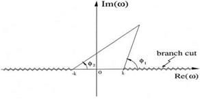
2 (Ф1 + Ф2)

That is, F(w) is the left side of Eq. (10.11). By tracing over the contour ABCDEFGH in the upper-half ю plane, it is easy to establish that the upper-half ю plane is mapped into the shaded region in the F plane as shown in Figure 10.5. The mapped region does not include the negative imaginary axis. Now X-1, on the right side of Eq. (10.11), is negative. This means that no value of ю in the upper-half ю plane would satisfy dispersion relation (10.11). Thus, the solutions of the initial value problem

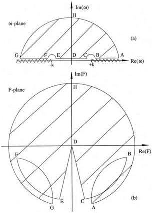Figure 10.5. Map of the upper-half ю plane in the F plane. (a) ю plane, (b) F plane.

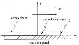
Figure 10.6. Schematic diagram show­ing a postulated zero-velocity fluid layer adjacent to an acoustically treated panel in the presence of a mean flow.

can only have ы with a negative imaginary part. These solutions are numerically stable.