Scattering of Acoustic Duct Mode at the Entrance and Exit of an Inlet Duct

At the entrance or the exit of an inlet duct, there is a surface discontinuity at the junction of the liner and hard wall (see Figure 10.12 or Figure 10.14). These junctions invariably cause significant spurious scattering of a propagating duct mode. The scattering is an artifact of discrete computation. It can be reduced by using a finer size mesh or by implementing the wave number truncation method of Section 9.6.

The governing equations of motion of the gas inside an inlet duct are the lin­earized dimensionless Euler equations. In cylindrical coordinates, these equations are

where M = u/a0 is the flow Mach number.

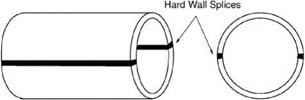Figure 10.13. Computational model of an inlet duct with two axial splices.

On the duct surface, the hard wall boundary condition is

1

‘ = 2’ V = °-

On the liner surface, the boundary condition is Eq. (10.19). At the left-hand junction of the computational model (Figure 10.12), the hard wall and liner boundary conditions can be combined to form a single boundary condition by means of the unit step function H(x). The combined boundary condition is

9 v d2v 9 p 9 p

RTT, – X-1v + X a? = H(x) { + Mi

Note: On the hard wall, x < 0, the H(x) function of boundary condition (10.47) is zero. This reduces the right side of the equation to zero. With the initial condition v = d v/д t = 0, the only solution is v = 0. In implementing the wave number truncation method, boundary condition (10.47) is replaced by

dv d2v 9 p d p

Rm – X-‘v+w=11 <x> і+Mі

where H(x), the truncated unit step function, is given by Eq. (9.67).

A cylindrical mesh, as shown in Figure 10.15, is used to compute the propaga­tion of acoustic modes upstream from the hard wall region on the right side of the

Figure 10.15. Cylindrical grid for duct acoustic mode computation. half the mesh lines are shown.

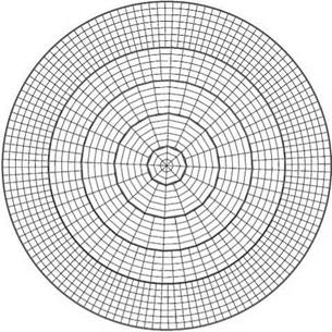inlet model of Figure 10.12 to the left side. A uniform size mesh in the axial direc­tion is used. Now, consider an incident duct mode with azimuthal mode number m = 26 and radial mode number n = 1 and a dimensionless angular frequency ^ = 0.573. For such an acoustic mode, an axial mesh with Ax = 0.008 will allow the computation to have more than 8 mesh points per axial wavelength. This is the mesh used in all the computations of this section unless explicitly stated otherwise. In the computation, the 7-point stencil dispersion-relation-preserving (DRP) scheme is used to approximate the derivatives. The multimesh-size, multitime-step DRP scheme (see Chapter 12) is used to march the solution in time. The duct wall bound­ary conditions (liner impedance, Z = 2 + i, time factor exp(-i^t)) are enforced by the ghost point method. Recently, this method has been used successfully by Tam et al. (2008) in their spliced liner study. On the left and right end of the computa­tional domain, a perfectly matched layer (PML) is implemented. The PML absorbs all the outgoing waves. The incident acoustic mode, which enters the computational domain on the right side, is introduced into the computation by the split-variable method as discussed in Section 9.1.

Figure 10.16 shows the axial distribution of computed acoustic energy flux (PWL) associated with an incident duct mode with azimuthal mode number 26 and other parameters as stipulated above. PWL is the total energy flux of all the sound waves in the duct. It is defined as 2n 1/2

J j ((1 + M2)pu + M(p2 + u2)) тйтйф, 00

where () is the time average. PWL(dB) = 10 log (PWL/PWLincidentwave). This form of energy flux was derived by Morfey (1971). Of particular interest here are the computed results near the left junction between acoustic liner and hard wall. In this region, the effect of scattering of spurious acoustic waves is most severe and

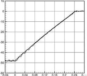
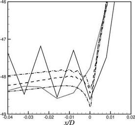Figure 10.16. Axial distribution of PWL. Incident wave has azimuthal mode number m = 26, radial mode num­ber n = 1, angular frequency Q = 0.573. Liner impedance Z = 2 + i

(time factor e-iQt).——— , Computed by

boundary condition (10.47), Ax = 0.008;

——- , computed by boundary condition

(10.47), Ax = 0.001; …… computed by

boundary condition (10.48), Ax = 0.008.

x/D

easily observable. The full line in this figure is the computed axial distribution of PWL using boundary condition (10.47) and axial mesh size 0.008. This curve exhibits strong spatial oscillations with a wavelength nearly equal to two axial mesh spacings. This is clear evidence of spurious scattering. The dotted line is the same computa­tion, but with a modified boundary condition (10.48). The computed distribution of PWL is smooth and free of spatial oscillations. This indicates that the wave number truncation method is indeed capable of removing spurious numerical scattering. To check the accuracy of the computed results by this method, a series of computations using boundary condition (10.47) is carried out with smaller and smaller axial mesh size Ax. Ax equals 1/4, 1/8, and 1/16 of the original mesh size used. The results near the left side liner-hard wall junction are shown in Figure 10.17 in an enlarged scale. As can be seen, as Ax is reduced, the computed result approaches that using boundary condition (10.48) but with a much larger Ax. The fact that there is good

Figure 10.17. Enlarged bottom left-hand corner of Figure 10.16. Computed by

boundary condition (10.47);——- , Ax =

0.008;——– , Ax = 0.002;———– , Ax =

0.001; — • • —, Ax = 0.0005; Computed

by boundary condition (10.48);…. Ax =

0.008.

agreement between results using much smaller Ax and boundary condition (10.47), and that using boundary condition (10.48) but much larger Ax, is evidence that the spatial oscillations of the full curve is of numerical origin. Further, it shows that the method of wave number truncation is effective and accurate. It also offers large savings in computer memory and CPU time.