Helmholtz’s Second Vortex Theorem

The second vortex theorem of Helmholtz’s states that:

“a vortex tube is always made up of the same fluid particles."

In other words, a vortex tube is essentially a material tube. This characteristic of a vortex tube can be represented as a direct consequence of Kelvin’s circulation theorem. Let us consider a vortex tube and an arbitrary closed curve c on its surface at time t0, as shown in Figure 5.30. By Stokes integral theorem, the circulation of the closed curve c is zero (that is, Dr/Dt = 0). The circulation of the curve, which is made up of the same material particles, still has the same (zero) value of circulation at a latter instant of time t.

y inverting the above reasoning, it follows from Stokes integral theorem that these material particles must be on the outer surface of the vortex tube.

If we examine smoke-rings, it can be seen that the vortex tubes are material tubes. The smoke will remain in the vortex ring and will be transported with it, so that it is the smoke itself which carries the vorticity. This statement holds under the restrictions of barotropy (that is, p = p(p), the density is a function of pressure only) and zero viscosity. The slow disintegration seen in smoke-rings is due to friction and diffusion. A vortex ring which consists of an infinitesimally thin vortex filament induces an infinitely large velocity on itself (similar to the horseshoe vortex), so that the ring would move forward with infinitely large velocity. The induced velocity at the center of the ring remains finite (as in horseshoe vortex). From Biot-Savart law, the induced velocity becomes:

_ Г Г2 h2dф _ Г 4 ж 0 h3 2 h

This velocity becomes infinitely large (that is, unrealistic) when the cross-section of the vortex ring is assumed to be infinitesimally small. For finite cross-section, the velocity induced by the ring on itself, that is, the velocity with which the ring moves forward remains finite. But in reality the actual cross-section of the ring is not known, and probably depends on how the ring was formed.

In practice we notice that the ring moves forward with a velocity which is slower than the induced velocity in the center. Also, it is well known that two rings moving in the same direction continu­ally overtake each other whereby one slips through the other in front. This phenomenon, illustrated in Figure 5.31, is explained by mutually induced velocities on the rings and formula given above for the velocity at the center of the ring.

In a similar manner it can be explained why a vortex ring towards a wall becomes larger in diameter and at the same time its velocity gets reduced. Also, the diameter decreases and the velocity increases when a vortex ring moves away from a wall, as illustrated in Figure 5.32.

To work out the motion of vortex rings the cross-section of vortex must be known. Further, for in­finitesimally thin rings the calculation fails because vortex rings, such as curved vortex filaments, induce large velocities on themselves. However, for straight vortex filaments, that is, for vortex filaments in two-dimensional flows, a simple description of the “vortex dynamics” for infinitesimally thin filaments is possible, since for such a case the self-induced translational velocity vanishes. We know that vortex filaments are material lines, therefore it is sufficient to calculate the paths of the fluid particles which carry the rotation in xy-plane perpendicular to the filaments, using:

Figure 5.32 Kinematics of a vortex ring near a wall.

that is, to determine the paths of the vortex centers. The induced velocity which a straight vortex filament at position xi induces at position x is known from Equation (5.49), that is:

v = ——- (cos a + cos 0) .

4nh

As we have seen, the induced velocity is perpendicular to the vector hi = ri = (x – xi), and therefore

hi

has the direction ez x ——, so that the vectorial form of Equation (5.41) reads as:

|hi|

Г

UR = ez x

2 n

For x ^ xi the velocity tends to infinity, but because of symmetry the vortex cannot be moved by its own velocity field, that is, the induced translational velocity is zero. The induced velocity of n vortices with the circulation Г (i = 1, 2, … n) is:

ur = ri<

2 n

If there are no internal boundaries, or if the boundary conditions are satisfied by reflection, as in Figure 5.32, the last equation describes the entire velocity field, and using dx/dt = u(x, t) or dxi/dt = ui(xi, t), the “equation of motion” of the kth vortex becomes:

For i = k, the induced translational velocity becomes zero, owing to symmetry, and hence excluded from the summation. Equation (5.58) gives the 2n relations for the path coordinates.

The dynamics of vortex motion have invariants which are analogous to the invariants of a point mass system on which no external forces act. The conservation of strengths of the vortices by Helmholtz’s theorem (^ Гк = constant) corresponds to mass conservation of total mass of the point mass system. When the Equation (5.58) is multiplied by Гк, summed over к and expanded, we get:

In the above equation, the terms on the right-hand side cancel out in pairs, and the equation reduces to:

On integration this results in:

k

The integration constants are written as xg, which is like a center of gravity coordinate (this is done here for dimensional homogeneity). Equation (5.59) states that:

“the center of gravity of the strengths of the vortices is conserved."

For a point mass system, by conservation of momentum, we have the corresponding law, namely: “the velocity of the center of gravity is a conserved quantity in the absence of external forces."

For ^ Гк — 0, the center of gravity lies at infinity, so that, for example, two vortices with Г1 — – Г2 must take a turn about a center of gravity point Pg which is at a finite distance, as shown in Figure 5.33.

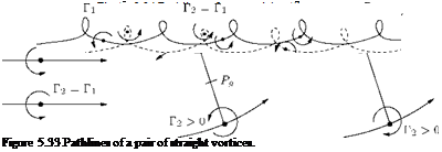The paths of the vortex pairs are determined by numerical integration of Equation (5.58). The paths will look like those shown in Figure 5.34.