Scattering by Thin Circumferential Splices

In this third example, the scattering of acoustic modes by a circumferential splices is considered. The computational model is shown in Figure 10.14. For this test case, the width of the circumferential splices is taken to be 2Ax. For this size splice, there are only 2 mesh points on the splice surface (Ax = 0.008).

Consider the function F(x) defined by

where xc is the location of the center of the splice and W is its width. By means of the F(x) function, the wall boundary condition for a liner with a single circumferential splice may be written as

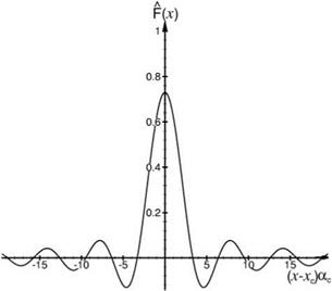Figure 10.21. The F (x) function. Wac = 2.5.

Now, the Fourier transform of F(x) is

Following the concept of the wave number truncated method, the high wave number components of Eq. (10.58) are to be removed at this stage. The truncated F(a) function is

e-laxc ( aw

F (a) = sin [H (a + ac) — H (a — ac)]. (10.59)

na 2

The inverse of F(a) is easily found to be 1

I7 (x) = [Si((x — xc + 0.5W )ac) — Si((x — xc — 0.5W )ac)]. (10.60)

n

A graph of I7(x) is given in Figure 10.21. The modified boundary condition to replace Eq. (10.57) is

Figure 10.22 shows the results of four computations for duct mode scattering by a circumferential splice of width 0.02 located between x = 0.11 and 0.13. The incident duct mode and the liner impedance are the same as in Section 10.6.1. The first three computations use boundary condition (10.57). The mesh size used in the first computation is Ax = 0.002. There is spurious acoustic scattering at the upstream end of the splice. The axial distribution of the acoustic PWL is the uppermost broken curve in Figure 10.22. The second and third computation use a mesh size of Ax = 0.0005 and 0.00025, respectively. It is clear from this figure that the spurious scattering diminishes with the use of a finer mesh. The fourth computation uses modified boundary condition (10.61) and a very coarse mesh of Ax = 0.008. This is 32 times the size of the finest mesh used. For this computation, there are only 2 mesh

Figure 10.22. Duct mode scattering by a circumferential splice of width 0.02. Inci­dent wave mode and liner impedance are the same as Figure 10.16. Compar­ison of transmitted PWL: computed by

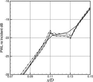boundary condition (10.61)—— Ax =

0.008; the following computed by bound­ary condition (10.57): Ax = 0.002,

…………… Ax = 0.0005, — • • — Ax =

0.00025.

points on the splice. The computed axial distribution of PWL is shown as the full line in Figure 10.22. For the transmitted PWL, which is one of the important quantities of the duct mode transmission computation, it is clear that the fourth computation using a mesh size 32 times larger gives almost identical results similar to those of the finest mesh. This example further illustrates the advantage of the wave number truncation method.

EXERCISES 10.1. Consider a single-frequency sound field of frequency О adjacent to an acous­tically treated panel or acoustic liner as shown in Figure 10.3. In other words, all the flow variables have the form p(x, y, z, t) = Re{p(x, y, z)e_iQt} when the solution has reached a time periodic state. Let the impedance of the liner be Z = R – iX. Verify that the following time-domain impedance boundary condition

d-P = R d-Vn _ xOvn

dt dt 11

yields the correct frequency-domain impedance boundary conditionp = Zvn.

Show by examining the dispersion relation of the acoustic field that boundary condition (A) is stable only when X < 0.

10.2. An acoustic wave train of frequency О = 1.6 kHz is sent down the normal incidence impedance tube shown in Figure 10.9. In dimensionless form, the incident wave is given by

Pincident = ^incident = cos[^(x _ t)] = Re _Ч •

The dimensionless resistance and reactance of the treatment panel are R = 0.18, X=-0.598, respectively. Compute the reflected wave train using boundary condition (A) of Problem 10.1. For this purpose, set up an incoming wave boundary condition on the left side of the computational domain. On the right side, use the ghost point
method to enforce the time-domain impedance boundary condition. Run your code long enough to attain a time periodic state before collecting numerical results.

Compare the pressure envelop inside the tube with that of the exact solution. The exact solution is

Preflected = Re {AeiQ(X+t} } , Mreflected = – Re {AeiQ(X+t} } ,

where A = (Z – 1)/(Z + 1). Note: Inside the normal incidence impedance tube the incident and the reflected wave train form a standing wave pattern. The maximum pressure amplitude at every point inside the tube form the pressure envelop.

10.3

Repeat Exercise 10.1 but replace boundary condition (A) by the following

Verify that time-domain impedance boundary condition (B) also leads to the correct frequency-domain impedance boundary condition p = Z vn. Show that (B) is stable only when X > 0.

10.4 Repeat Exercise 10.2 but at a higher frequency of 3 kHz. At this frequency, the resistance and reactance of the treatment panel are R = 0.18, X = 0.678. Use time-domain impedance boundary condition (B) in your computation. Compare your computed pressure envelop with the exact solution.