Additional Constraint on Optimized Extrapolation

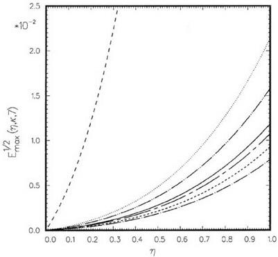
Figure 11.6 indicates that the extrapolation error for high wave numbers, particularly for a Ax near n, is very large. This means that, in a large-scale computation, the high wave number components can be greatly amplified by the extrapolation process. This observation suggests that it is this numerical error amplification mechanism that is responsible for the often encountered numerical instability associated with extrapolation. From this point of view, it would be desirable to keep the local error at a Ax = n and over the high wave number range smaller. This may be done by imposing an additional constraint on the optimization process. Suppose it is desired to fix the extrapolated error El1o/c2al of the function at a Ax = n to be a prescribed value, say, h(n). For this purpose, an additional condition,

Figure 11.7. Dependence of maximum local error (maximized over 0 < a Ax < 0.85) on n for the case N = 7…………. , к = 0.8;——– , к = 0.85; — —, к = 0.95;——— , к = 1.0;………………………. , к = 1.05;———— , к = 1.1;——– , Lagrange polynomials extrapolation.

is imposed. The first term of Eq. (11.21) is equal to the extrapolated value of the simple wave function fa(x) of Eq. (11.11) at aAx = n. Thus, for all intents and purposes, it is equal to the square root of the local error. By specifying the function h(n), one stipulates the maximum error allowed at aAx = n. Extensive numerical experiments have found that a good choice of h(n) is

h (n) = 1.0 + 19n. (11.22)

Upon including Eq. (11.21) as an additional constraint, the Lagrangian function to be minimized is

The conditions for minimization are as follows:

dS = 0, j = 0, 1, 2,…, (N – 1), dX = 0, dX = 0. (11.24)

dSj dX dx

Eq. (11.24) may be recast into a matrix system as follows: к sin к sin 2к 2 sin 3к 3 sin 4к 4 sin[(N-1)к] N-1 1 2 1 ” 2 sin к к sin к sin 2к 2 sin3K 3 sin[(N-2)к] ‘ ‘ N-2 1 2 1 2 sin 2к 2 sin к к sin к sin 2к 2 sin[(N-3)к] ‘ ‘ N-3 1 2 1 2 sin3K 3 sin2K 2 sin к к sin к sin[(N-4)к] N-4 1 2 1 2 sin[(N – 1)к] N-1 sin[(N-2)к] N-2 sin[(N-3)к] N-3 • • к 1 2 (-1)N-12 1 1 1 1 1 • • 1 1 0 1 -1 1 -1 1 • • (-1)N-1 0 0

Г S ]		~ sin^) ” n
S1		n+1
S2		sin(n+2)к n+2
S3	=	sin(n+3)к n+3
SN-1 X		sin(n+N-1)к n+N-1 1
ft		h(n)

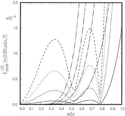
Eq. (11.25) may be solved easily by a standard matrix equation solver. Once S;-’s are found, the local error £local can be calculated. Figure 11.8 shows the variation of Еоы with wave numbers a Ax for к = 0.85, N = 7 at four values of n. For a Ax < 0.8 or 8 mesh points or more per wavelength, the maximum extrapolation error is less than

1.5 percent. Shown in this figure also are the local errors of the Lagrange polynomials extrapolation method. It is evident that for a Ax > 0.6, the error is huge. Figure 11.9 shows an identical plot but covers the entire range of wave numbers. Near a Ax = n, there is significant difference in the errors between the two extrapolation procedures. For instance, for n= 1.0, the Lagrange polynomials method has an error about six times larger than that of the optimized scheme. One would, therefore, expect that the improved optimized scheme is less likely to induce numerical instability.

Figures 11.10 to 11.13 provide similar information as Figures 11.8 and 11.9 at stencil sizes of 5 and 8. They illustrate the effect of using a smaller or larger extrapolation stencil. Generally speaking, the use of a larger stencil reduces the error in the low wave number range but increases the error at high wave numbers. This is a piece of useful information in deciding the proper stencil size to use.

As an example that the added constraint in the optimized extrapolation method does reduce numerical instability, the one-dimensional acoustic wave propagation and reflection problem of Figure 11.2 is again considered. Now the computation is

Figure 11.8. Local error as a function of wave number using the optimized extrapolation method with an added constraint. к = 0.85, N = 7.

П optimized extrapolation Lagrange polynomials extrapolation

0.25—————- ————————————-

0.50 ——— ————————————-

0.75 ………… ………………………………………………

1.00 ————— —————————————- repeated using the optimized extrapolation scheme to find the value of u at the wall, x = n,; i. e.,

6

£>_ jSj (n) = 0. (11.26)

j=0

It can be shown analytically and demonstrated computationally (see Tam and Kurbatskii, 2000) that there is no boundary instability. In other words, the opti­mized scheme with the additional constraint has effectively eliminated the boundary instability mode created by numerical extrapolation using the Lagrange polynomials method.