Optimized Interpolation Method

In this section, a wave number analysis of interpolation error is performed. At the same time, an optimized interpolation procedure is formulated. Interpolation is generally a numerically stable operation incurring relatively little error. For this

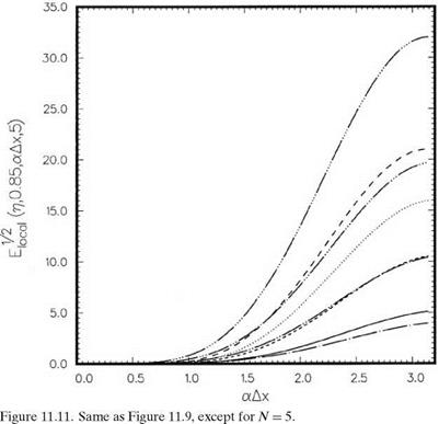
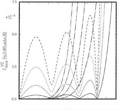
Figure 11.9. Same as Figure 11.8, except the full wave number range is shown.

0.0 0.1 0.2 0.3 0.4 0.5 0,6 0.7 0.8 0.9 1.0 о;Дх

Figure 11.13. Same as Figure 11.9, except for N = 8.

reason, one can only expect a relatively small improvement by using an optimized scheme.

Consider an N-point interpolation stencil as shown in Figure 11.14. Let x0 be the first point of the stencil. The other stencil points are located at Xj = x0 – jAx (j = 1 to (N – 1)). Suppose the interpolation point is in the Kth interval of the stencil at a distance of nAx to the right of xK. The interpolation formula is

N-1

Ev (xj )•

j=0

As before, the local interpolation error, £local, is defined as the square of the absolute value of the difference between the left and the right sides of Eq. (11.27) when the single Fourier component of Eq. (11.11) is substituted into the

Now, the interpolation coefficients Sj are chosen so that E is a minimum sub­jected to the condition that there is no error for zero wave number. The zero wave number condition may be written as

N—1

The Lagrangian function of this constrained minimization problem is

Л Sj = 1

j=0

The linear system Eq. (11.33) may be rewritten in a matrix form similar to Eq. (11.19). The matrix equation can be solved easily to provide the interpolation coefficients, Sj (j = 0,1, 2,…, (N—1)).

The local interpolation error Elocal as a function of wave number a Ax depends on a number of parameters. They are N (the stencil size), K (the interval number), n (the distance to the mesh point), and the free parameter к. Numerical results are now provided to offer an idea on the magnitude of the error and how it is influenced by the various parameters.

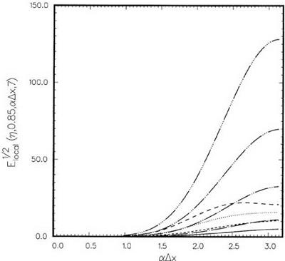
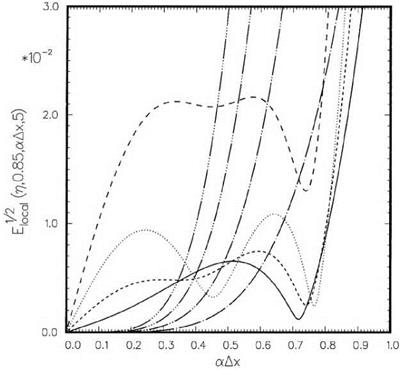
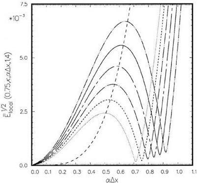
Consider first the effect of N, the size of the stencil. Figure 11.15 shows the distribution of Elocal in wave number space for n= 0.75 using only two interpolation points, N = 2. This is a very special case. The parameter к appears to have a negligible effect on the local error. In addition, the optimized scheme yields almost identical results as the Lagrange polynomials interpolation. The error is relatively large in the high wave number range, but relatively small at low wave numbers. The interpolation point will now be kept in the first interval of the stencil, i. e., K = 1, but the stencil size is allowed to increase. Figures 11.16 and 11.17 show the local error distributions as functions of wave number at various values of к with N = 4 or four interpolation points. On comparison with Figure 11.15, it is clear that, by increasing the size of the stencil, the error in the low wave number range drops rapidly. At the same time, the error in the high wave numbers increases. Figures 11.18 and 11.19 provide the results for an even larger stencil, N = 7. In this case, the low wave number error becomes negligible, but the error in the neighborhood of a Ax = n is much larger.

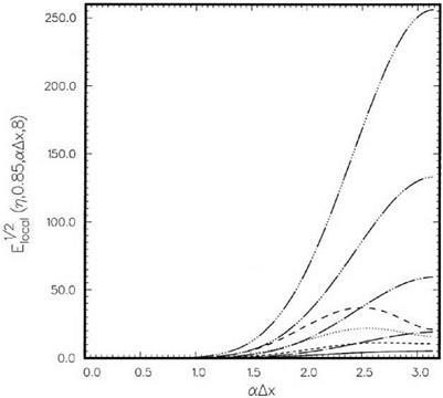
If the interpolation point lies in the interior of a large stencil, one intuitively expects much smaller error than when it is located at the first interval. Figures 11.20 and 11.21 show the numerical results for N = 7, n= 0.75, and K = 2. Figures 11.22 and 11.23 show the corresponding results for K = 3. These results completely confirm the intuitive expectation. Over the long wave range, a Ax < 0.9, there is hardly any error when the interpolation point lies in the center interval for large N

Figure 11.16. Dependence of local interpolation error on wave number. N = 4, K = 1, n = 0.75………….. , к = 0.85;——— , к = 0.9;——— , к = 0.95;———- , к = 1.0;——— , к = 1.05; ———— , к = 1.1;——– , Lagrange polynomials interpolation.

The effect of the distance of the interpolation point from the stencil point, namely, the magnitude of n will now be considered. Figures 11.24 and 11.25 give the local errors for n= 0.25. The values of the other parameters are the same as those of Figures 11.18 and 11.19. As readily seen, the two sets of figures are about the same. This indicates that n has a relatively small effect on the local error.

Finally, the effect of free parameter к is considered. After reviewing and compar­ing all the numerical results, it is found that a good overall choice for this parameter is 1.0. This value of к provides a large range of low wave numbers over which the interpolation error is small. At the same time, the error at high wave numbers is still numerically small. In most large-scale computations, the high wave number com­ponents will remain unresolved. They are the spurious numerical waves, which are suppressed by the inclusion of artificial selective damping or filtering. As a result, the amplitude of the high wave number components is expected to be small. Any amplification by the interpolation process would still be small. They should not be a concern except in unusual circumstances.