Our heavyweight helicopter equal in the world does not have
In Rostov started production of the most load-lifting rotary-wing car The Russian holding «Helicopt[...]

Everything about aircrafts and helicopters. News and events in aviation worldwide. Civil, transportation, military helicopters and airplanes.

Everything about aircrafts and helicopters. News and events in aviation worldwide. Civil, transportation, military helicopters and airplanes.

Everything about aircrafts and helicopters. News and events in aviation worldwide. Civil, transportation, military helicopters and airplanes.

Everything about aircrafts and helicopters. News and events in aviation worldwide. Civil, transportation, military helicopters and airplanes.


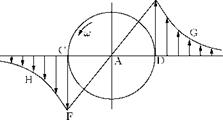
Consider a circular vortex of strength у, defined by:
2ny = circulation = nazf.
|
E
Figure 5.48 Velocity distribution along a diameter of a circular vortex. |
Thus,
1 2r Y = 2
Therefore, the velocity induced by this circular vortex is:
V’ = Y —2, r < a
a
т/ y
V = —, r > a. r
The velocities at all points of a diameter are perpendicular to that diameter, hence the extremities of the velocity vectors at the different points of the diameter will lie on a curve which gives the velocity distribution as we go along the diameter from —to to +to, as shown in Figure 5.48.
From points between C and D the velocity variation (along a diameter) is a straight line EAF, the variation from C to —to and D to +to is part of a rectangular hyperbola whose asymptotes are the diameter CD and the perpendicular diameter through the center A. The ordinates DE and CF, each represent the velocity у/a. Thus, if for a circular vortex of constant strength y, as the radius a decreases, DE will increase. Therefore, in the limit when a ^ 0 the velocity variation will consist of the rectangular hyperbola with the asymptote perpendicular to CD.
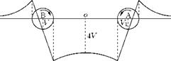
Now let us study the field of two identical circular vortices of radius a but with opposite vorticity (Z and – Z) at a finite distance apart, as shown in Figure 5.49. If the distance between their center BA is sufficiently large compared to a, as a first approximation, we can suppose that the vortices do not interfere and remain circular. For such a case their velocity fields may be compounded by the ordinary law of vector addition. The effect on the velocity distribution plot of A will reduce all the velocities at points near A on the diameter CD (see Figure 5.48) by approximately v = y/BA. The general shape of the velocity distribution plot for the pair of vortices will be as shown in Figure 5.49.
|
Figure 5.49 General shape of the velocity distribution for a pair of vortices. |
It can be seen that the center of each vortex is now in the field of velocity induced by the other and would therefore move with velocity v in the direction perpendicular to AB. Thus the vortices are no longer at rest, but move with equal uniform velocity, remaining at a constant distance apart. This is an application of the theorem that “a vortex induces no velocity on itself.” The vortices and velocity field shown in Figure 5.49 has its application to the study of the induced velocity due to the wake of a monoplane aerofoil at a distance behind the trailing edge.