The natural modes of motion

For small-amplitude stability analysis, helicopter motion can be considered to com­prise a linear combination of natural modes, each having its own unique frequency, damping and distribution of the response variables. The linear approximation that al­lows this interpretation is extremely powerful in enhancing physical understanding of the complex motions in disturbed flight. The mathematical analysis of linear dynamic systems is summarized in Appendix 4A, but we need to review some of the key results to set the scene for the following discussion. Free motion of the helicopter is described by the homogeneous form of eqn 4.41

x – Ax = 0 (4.117)

subject to initial conditions

x(0) = x0

The solution of the initial value problem can be written as

x(t) = W diag [exp(X;t)] W-1xo = Y(t)xo (4.119)

The eigenvalues, k, of the matrix A satisfy the equation

det[kI – A] = 0 (4.120)

and the eigenvectors w, arranged in columns to form the square matrix W, are the special vectors of the matrix A that satisfy the relation

Aw i = ki wi (4.121)

The solution can be written in the alternative form

n

x(t) = ^2(vTX0) exp(kit)wi (4.122)

i =0

where the v vectors are the eigenvectors of the transpose of A (columns of W-1), i. e.,

AT vj = k j vj (4.123)

The free motion is therefore shown in eqn 4.122 to be a linear combination of natural modes, each with an exponential character in time defined by the eigenvalue, and a distribution among the states, defined by the eigenvector.

The full 6 DoF helicopter equations are ninth order, usually arranged as [u, w, q, 9, v, р, ф,г, ф], but since the heading angle ф appears only in the kine­matic equation relating the rate of change of Euler angle ф to the fuselage rates p, q, r, this equation is usually omitted for the purpose of stability analysis. Note that, for the ninth-order system including the yaw angle, the additional eigenvalue is zero (there is no aerodynamic or gravitational reaction to a change in heading) and the associated eigenvector is {0, 0, 0, 0, 0, 0, 0, 0, 1}.

The eight natural modes are described as linearly independent so that no single mode can be made up of a linear combination of the others and, if a single mode is excited precisely the motion will remain in that mode only. The eigenvalues and eigenvectors can be complex numbers, so that a mode has an oscillatory character, and such a mode will then be described by two of the eigenvalues appearing as conjugate complex pairs. If all the modes were oscillatory, then there would only be four in total. The stability of the helicopter can now be discussed in terms of the stability of the individual modes, which is determined entirely by the signs of the real parts of the eigenvalues. A positive real part indicates instability, a negative real part stability. As one might expect, helicopter handling qualities, or the pilot’s perception of how well a helicopter can be flown in a task, are strongly influenced by the stability of the natural modes. In some cases (for some tasks), a small amount of instability may be acceptable; in others it may be necessary to require a defined level of stability. Eigenvalues can be illustrated as points in the complex plane, and the variation of an eigenvalue with some flight condition or aircraft configuration parameter portrayed as a root locus. The eigenvalues are given as the solutions of the determinantal eqn 4.120, which can also be written in the alternate polynomial form as the characteristic equation

Xn + an—1Xn 1 +•••+ ai^i + ao = 0 (4.124)

or as the product of individual factors

(X – Xn)(X – Xn-)(……….. )(X – X1) = 0 (4.125)

The coefficients of the characteristic equation are nonlinear functions of the stability derivatives discussed in the previous section. Before we discuss helicopter eigenvalues and vectors, we need one further analysis tool that will prove indispensable for relating the stability characteristics to the derivatives.

Although eigenanalysis is a simple computational task, the eighth-order system is far too complex to deal with analytically, and we need to work analytically to glean any meaningful understanding. We have seen from the discussion in the previous section that many of the coupled longitudinal/lateral derivatives are quite strong and are likely to have a major influence on the response characteristics. As far as stability is concerned however, we shall make a first approximation that the eigenvalues fall into two sets – longitudinal and lateral, and append the analysis with a discussion of the effects of coupling. Even grouping into two fourth-order sets presents a formidable analysis problem, and to gain maximum physical understanding we shall strive to reduce the approximations for the modes even further to the lowest order possible. The conditions of validity of these reduced order modelling approximations are described in Appendix 4A where the method of weakly coupled systems is discussed (Ref. 4.24). In the present context the method is used to isolate, where possible, the different natural modes according to the dominant constituent motions. The partitioning works only when there exists a natural separation of the modes in the complex plane. Effectively, approximations to the eigenvalues of slow modes can be estimated by assuming that the faster modes behave in a quasi-steady manner. Likewise, approximations to the fast modes can be derived by assuming that the slower modes do not react in the fast time scale. A second condition requires that the coupling effects between the contributing motions are small. The theory is covered in Appendix 4A and the reader is encouraged to assimilate this before tackling the examples described later in this section.

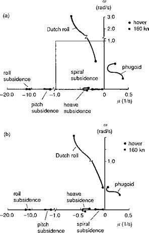
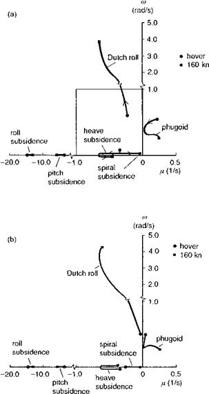
Figures 4.23, 4.24 and 4.25 illustrate the eigenvalues for the Lynx, Bo105 and Puma, respectively, as predicted by the Helisim theory. The pair of figures for each aircraft shows both the coupled longitudinal/lateral eigenvalues and the corresponding uncoupled values. The predicted stability characteristics of Lynx and Bo105 are very similar. Looking first at the coupled results for these two aircraft, we see that an unstable phugoid-type oscillation persists throughout the speed range, with time to double amplitude varying from about 2.5 s in the hover to just under 2 s at high speed. At the hover condition, this phugoid mode is actually a coupled longitudinal/lateral oscillation and is partnered by a similar lateral/longitudinal oscillation which develops into the classical Dutch roll oscillation in forward flight, with the frequency increasing strongly with speed. Apart from a weakly oscillatory heave/yaw oscillation in hover, the other modes are all subsidences having distinct characters at hover and low speed – roll, pitch, heave and yaw, but developing into more-coupled modes in forward flight, e. g., the roll/yaw spiral mode. The principal distinction between the coupled (Figs 4.23(a) and 4.24(a)) and the uncoupled (Figs 4.23(b) and 4.24(b)) cases lies in the

Fig. 4.23 Loci of Lynx eigenvalues as a function of forward speed: (a) coupled; (b) uncoupled

stability of the oscillatory modes at low speed where the coupled case shows a much higher level of instability. This effect can be shown to be almost exclusively due to the coupling effects of the non-uniform inflow caused by the change in wake angle induced by speed perturbations; the important derivatives are Mv and Lu, caused by the coupled rotor flapping response to lateral and longitudinal distributions of first harmonic inflow respectively. The unstable mode is a coupled pitch/roll oscillation with similar ratios of p to q and v to u, in the eigenvector.

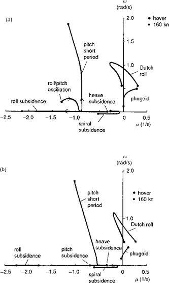
The Puma comparison is shown in Figs 4.25(a) and (b). The greater instability for the coupled case at low speed is again present, and now we also see the short­term roll and pitch subsidences combined into a weak oscillation at low speed and hover. As speed increases the coupling effects again reduce, at least as far as stability is concerned. Here we are not discussing response and we should expect the coupled response characteristics to be strong at high speed, we shall return to this topic in the next chapter. At higher speeds the modes of the Puma, with its articulated rotor,

Fig. 4.24 Loci of Bo105 eigenvalues as a function of forward speed: (a) coupled; (b) uncoupled

resemble the classical fixed-wing set: pitch short period, phugoid, Dutch roll, spiral and roll subsidence. An interesting feature of the Puma stability characteristics is the dramatic change in stability of the Dutch roll from mid- to high speed. We shall discuss this later in the section.

Apart from relatively local, although important, effects, the significance of cou­pling for stability is sufficiently low to allow a meaningful investigation based on the uncoupled results, and hence we shall concentrate on approximating the characteristics

Fig. 4.25 Loci of Puma eigenvalues as a function of forward speed: (a) coupled; (b) uncoupled

illustrated in Figs 4.23(b)-4.25(b) and begin with the stability of longitudinal flight dynamics.