Time Marching Stencil

The time marching step, ft, is constrained by the numerical stability or accuracy requirements of a computation scheme. In general, the stability or accuracy require­ments link ft directly to the mesh size fx. Thus, in a region with large mesh size, a larger ft may be used. When more than one mesh size is used, the optimum strategy is to use the largest time step permissible in each region. It follows, if the mesh size changes by a factor of 2 in adjacent domains, the time step should also change by the same ratio. Figure 12.2 shows the time levels of the computation in the mesh – size-change buffer region. In the fine mesh region on the left, the time step is ft. In the coarse mesh region on the right, the time step is 2ft. Effectively, the fine mesh region is computed twice as often as the coarse mesh region.

Suppose the solution is known at time level n (see Figure 12.2), the solution in the fine mesh region may be advanced by a time step At to time level (n + 1 /2) in the usual way. Once this is completed, the next step is to advance the solution to time level (n + 1) in both the fine and coarse mesh regions. It is straightforward to carry out this step in the coarse mesh region by using the solution on time levels n, (n – 1), (n – 2), and (n – 3). However, for points in the buffer region on the fine mesh side, the stencils extend into the coarse mesh region. There is no information at the (n + 1/2) time level at these points on the coarse mesh side. To provide the needed information of the solution, it is necessary to compute the solution at the time level (n + 1 /2) for the first two rows or columns of the mesh point on the coarse mesh side based on the solution at time levels n, (n – 1), (n – 2), and (n – 3). To advance the solution by a half time step as shown in Figure 12.2, the following four-level scheme may be used:

where К = du/dt is given by the governing equation, and (l, m) are the spatial indices.

(e-iaAt -1) 3 Ul, m (2At )Y^ b*e2ijaAt j=0 1

To find the stencil coefficients b* of Eq. (12.9), one may consider u to be made up of a Fourier spectrum of simple harmonic components of the form e-iat, where a is the angular frequency. The effect of time marching algorithm (12.9) on each Fourier component of frequency a may be analyzed by substituting ufm = ulm (t) = Ae-lan(2At) into Eq. (12.9). It is easy to find

Since d(u m/dt)=iaul m, the factor, on the right side of Eq. (12.10), multiplying U m, must be equal to – ia, where a is the angular frequency of the time marching finite difference scheme. Thus, one finds that

i(e-iaAt -1)

3

2 b*e2i1aAt

1=0 1

There are four coefficients, namely, b*0, b*, b2, and b. Here, the condition that a ~ a be accurate to order (At)[15] is imposed. On expanding Eq. (12.11) by the Taylor series, it is straightforward to find that the four coefficients are related by the following three conditions:

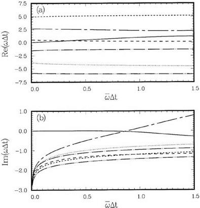
Figure 12.7. The dependence of the seven roots of юAt on a) At.

There is no loss of generality regarding b0 as the remaining free parameter. The value of b0 is chosen so that ю is a good approximation of ю over the frequency band – X < юAt < X. This is done by minimizing the integral as follows:

A

E(bo) = j {a[Re(«At) — юAt]2 + (1 — a)[Im(«At)]2} d(o^At), (12.15)

-A

where a is the weight parameter. The condition for minimization is dE/db0 = 0.

A numerical study of the real and imaginary parts of («At — rnAt) for different choices of X and a has been carried out. Based on the results of this study, the values X = 0.5 and a = 0.42 are recommended for use. For this choice of parameters, the optimized coefficients are as follows:

b0 = 0.773100253426 b = —0.485967426944 b2 = 0.277634093611 b3 = —0.064766920092.

For a given «At, Eq. (12.11) yields seven roots of юAt. As in the original DRP scheme, only one of the roots yields the physical solution. All the other roots are spurious and should be damped if the scheme is to be stable. Figure 12.7 shows
the dependence of the roots on «At. The scheme is stable if «At < 0.88. If «At is restricted to less than or equal to 0.19, then the damping rate, Im(«At), is less than 0.78 x 10-5, which is quite small. The accuracy of this scheme when restricted to this range is comparable to that of the standard DRP scheme.