AIRCRAFT RECONFIGURABLE/RESTRUCTURABLE CONTROL SYSTEM

A typical FTR control system would consist of actuators, sensors, computer systems, data acquisition systems, and often mechanical, hydraulic, pneumatic, electronic devices and systems [9-11]. A fault-tolerant flight-control system (FTFCS) is expected to perform the task of failure detection, identification, and accommodation of actuator and general failures. FTFCS is also useful for UAVs and MAVs. In a reconfigurable FTFCS, a full set of possible failures for different control surfaces and other probable faults is predefined. The required changes in control gains are computed offline in advance and stored in OBC for subsequent online usage. This approach requires an extensive design to consider all possible failure modes and hence a large storage space in OBC is required. In restructurable FTFCS, the required control laws are restructured online based on some identified system/fault parameters, particularly damage to a wing or control surface. ANNs and fuzzy logic find a good use for this type FTFCS. For FTFCSs, two aspects are important: (1) detection and identification of actuator fault and (2) failure accommodation. For an FBW aircraft, fault-tolerant capacity requires an increase in the number of independent control surfaces. This selection depends on: (1) control effectiveness (Cm), (2) increased aircraft complexity and cost, (3) weight constraint, (4) aerody­namic drag force, and (5) aircraft type. When any type of control surface failure occurs, the coupling between longitudinal and lateral-directional dynamics is of great concern, since this might lead to loss of stability of the vehicle. In many of these studies an accurate postfailure aerodynamic model for simulation is required. From Equation 4.6 we can guess that a damage of a control surface would cause instantaneous changes in its aerodynamic characteristics. Neglecting the effect on the axial forces, the net effect of the damage of the control surface would normally be the reduction in the relative normal force coefficient.

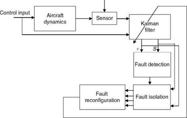
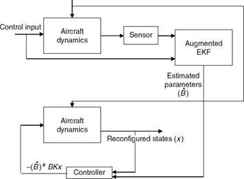
Sensors and actuators play a vital role in the control mechanisms of various aerospace vehicles/systems. Problems arise when a particular sensor stops working properly due to an unknown internal fault or component impairment or any cata­strophic disturbance from an external source. In that case, the whole architecture of the control system becomes hampered. There is an urgent requirement for a model that detects the failed sensor as quickly as possible and reconfigures the damaged architecture so that the controlling mechanism continues to deliver desired results without any alterations. Timely detection and adjustment of the system to cope with these uncertainties are highly desirable. This process of identification and reconfig­uration is known as sensor fault detection, isolation, and accommodation (SFDIA). The two most popular methods for SFDIA are model – and non-model-based approaches. These techniques are based on analysis of residuals between measured and predicted plant states. In the model-based technique, the algorithms commonly used are RKF (robust Kalman filter) [11], MMAE (multiple model adaptive estima­tor), and IMM (interacting multiple model). In the non-model-based approach, neural networks and fuzzy logic are used to predict the plant responses and this in conjunction with the measured states is subsequently used to detect and isolate the sensor fault. The other potential cause for hampered aircraft performance is its faulty actuator. The process of detection, isolation, and reconfiguration of actuator faults is known as AFDIA. In this case, the strategy is to pinpoint the cause of failure and then appropriately reconfigure the flight-control system such that the impaired aircraft can be made flyable.

Figures 8.10 and 8.11 show the architectures used for fault detection, isolation, and reconfiguration for sensor and actuator, respectively. For data simulation, the longitudinal dynamics of aircraft control system are considered. The state-space formulation of the longitudinal motion of aircraft in continuous-time domain is as follows:

x = Ax + Buc + Gwn (8.26)

Here, x = [u, w, q, U] are the physical variables corresponding to aircraft longitudinal motion. wn is zero mean white Gaussian process noise.

The equation used to model the sensor is given by

Zm(k) = Hx + v (8.27)

The observation matrix H is an identity matrix with the dimension 4 x 4. The measurements can be obtained with a sampling time interval T equal to 0.01 s.