Appendix 4A The Analysis of Linear Dynamic Systems (with Special Reference to 6 DoF Helicopter Flight)

The application of Newton’s laws of motion to a helicopter in flight leads to the assembly of a set of nonlinear differential equations for the evolution of the aircraft response trajectory and attitude with time. The motion is referred to an orthogonal axes system fixed at the aircraft’s cg. In Chapter 3 we have discussed how these equations can be combined together in first-order vector form, with state vector x(t) of dimension n, and written as

x = F(x, u, t) (4A.1)

The dimension of the dynamic system depends upon the number of DoFs included. For the moment we will consider the general case of dimension n. The solution of eqn 4A.1 depends upon the initial conditions of the motion state vector and the time variation of the vector function F(x, u, t), which includes the aerodynamic loads, gravitational forces and inertial forces and moments. The trajectory can be computed using any of a number of different numerical integration schemes which time march through a simulation, achieving an approximate balance of the component accelerations with the applied forces and mo­ments at every time step. While this is an efficient process for solving eqn 4A.1, numerical integration offers little insight into the physics of the aircraft flight behaviour. We need to turn to analytic solutions to deliver a deeper understanding between cause and effect. Unfortunately, the scope for deriving analytic solutions of general nonlinear differential equations as in eqn 4A.1 is extremely limited; only in special cases can functional forms be found and, even then, the range of validity is likely to be very small. Fortunately, the same is not true for linearized versions of eqn 4A.1, and much of the understanding of complex dynamic aircraft motions gleaned over the past 80 years has been obtained from studying linear approximations to the general nonlinear motion. Texts that provide suitable background reading and deeper understanding of the underlying theory of dynamic sys­tems are Refs 4A.1-4A.3. The essence of linearization is the assumption that the motion can be considered as a perturbation about a trim or equilibrium condition; provided that the perturbations are small, the function F can usually be expanded in terms of the motion and control variables (as discussed earlier in this chapter) and the response written in the form

x = Xe + Sx (4A.2)

where Xe is the equilibrium value of the state vector and Sx is the perturbation. For conve­nience, we will drop the S and write the perturbation equations in the linearized form

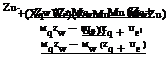
x – Ax = Bu(t) + f(t) (4A.3)

where the (n x n) state matrix A is given by

and the (n x m) control matrix B is given by

and where we have assumed without much loss of generality that the function F is differen­tiable with all first derivatives bounded for bounded values of flight trajectory x and time t.

We write the initial value at time t = 0, as x(0) = xo (4A.6) The flight state vector x is a vector in n-dimensional space, where n is the number of independent components. As an example of eqn 4A.3, consider the longitudinal motion of the helicopter, uncoupled from lateral/directional dynamics, and with rotor and other ‘higher’ DoFs subsumed into the fourth-order rigid body equations. The linearized equations of motion for perturbations from straight flight can be written in the form
u ‘Xu Xw Xq – We -g cos ®e " u ‘X в0 Xels’ d w Zu Zw Zq + Ue -g sin ®e w Z в0 Ze1s dt q Mu Mw Mq 0 q M0 M*s в 0 0 1 0 в 0 0
eo(t) &1s(t) (4A.7)
Xw Zw Mw 0
[wg(t)]
+
Longitudinal motion is here described by the four-vector with elements u (forward velocity perturbation from trim Ue), w (normal velocity perturbation from trim We), q (pitch rate) and в (pitch attitude perturbation from trim @e). As an illustration of the forcing function, we have included both collective and cyclic rotor controls and a normal gust field wg. In this tutorial-style appendix, we will use the example given by eqn 4A.7 to illustrate the physical significance of theoretical results as they are derived. Equation 4A.3 is valid for calculating the perturbed responses from a trim point, but in the homogeneous form, with no forcing function, it can be used to quantify the stability characteristics for small motions of the nonlinear dynamic system described by eqn 4A.1. This is a most important application and underpins most of the understanding of flight dynamics. The free motion solutions of eqn 4A.3 take the form of exponential functions; the signs of the real parts determine the stability with positive values indicating instability. The theory of the stability of motion for linear dynamic systems can be most succinctly expressed using linear algebra and the concepts of eigenvalues and eigenvectors. Consider the free motion given by
X – Ax = 0	(4A.8)
(4A.9)
so that eqn 4A.8 can be written as
(4A.10)
y – Ay = 0
with
A = W-1 AW
(4A.11)
For a given matrix A, there is a unique transformation matrix W that reduces A to a canonical form, A, most often diagonal, so that eqn 4A.10 can usually be written as a series

of uncoupled equations

Уі – kyi = 0, i = 1, 2,…, n (4A.12)

with solutions

Уі = У^к‘ (4A.13)

Collected together in vector form, the solution can be written as

y = diag [exp (X, t)] У0 (4A.14)

Transforming back to the flight state vector x, we obtain

x(t) = W diag [exp (kit)] W-1×0 = Y(t)x0 = exp(At)x0 (4A.15)

where the principal matrix solution Y(t) is defined as

Y(t) = 0, t < 0, Y(t) = W diag [exp(X, t)] W-1, t > 0 (4A.16)

We need to stop here and take stock. The transformation matrix W and the set of numbers X have a special meaning in linear algebra; if wi is a column of W then the pairs [wi, Xi ] are the eigenvectors and eigenvalues of the matrix A. The eigenvectors are special in that when they are transformed by the matrix A, all that happens is that they change in length, as given by the equation

Aw і = Xi Wi (4A.17)

No other vectors in the space on which A operates are quite like the eigenvectors. Their special property makes them suitable as basis vectors for describing more general motion. The associated eigenvalues are the real or complex scalars given by the n solutions of the polynomial

det[XI – A] = 0 (4A.18)

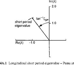
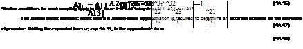
The free motion of a helicopter is therefore described by a linear combination of simple exponential motions, each with a mode shape given by the eigenvector and a trajectory envelope defined by the eigenvalue. Each mode is linearly independent of the others, i. e., the motion in a mode is unique and cannot be made up from a combination of other modes. Earlier in this chapter, a full discussion on the character of the modes of motion and how they vary with flight state and aircraft configuration was given. Below, in Figs 4A.1 and 4A.2, we illustrate the eigenvalue and eigenvector associated with the longitudinal short period mode of the Puma flying straight and level at 100 knots; we have included the modal content of all eight state vector components u, w, q, в, v, p, ф, r. The eigenvalue, illustrated in Fig. 4A.1, is given by

Xsp = -1.0 ± 1.3i

(4A.20)

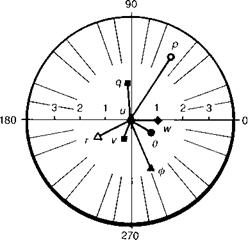
Fig. 4A.2 Longitudinal short period eigenvector – Puma at 100 knots

The short period frequency is given by

asp = Im(ksp) = 1.3 rad/s (4A.21)

and, finally, the damping ratio is given by

zsp = – Re(Xsp) = 0.769 (4A.22)

asp

We choose to present the angular and translational rates in the eigenvectors shown in Fig. 4A.2 in deg/s and in m/s respectively. Because the mode is oscillatory, each component has a magnitude and phase and Fig. 4A.2 is shown in polar form. During the short period oscillation, the ratio of the magnitudes of the exponential envelope of the state variables remains constant. Although the mode is described as a pitch short period, it can be seen in Fig. 4A.2 that the roll and sideslip coupling content is significant, with roll about twice the magnitude of pitch. Pitch rate is roughly in quadrature with heave velocity.

The eigenvectors are particularly useful for interpreting the behaviour of the free response of the aircraft to initial condition disturbances, but they can also provide key information on the response to controls and atmospheric disturbances. The complete solution to the homogeneous eqn 4A.3 can be written in the form

or expanded as

(4A.24)

where v is the eigenvector of the matrix AT, i. e., vT are the rows of W 1 (VT = W 1) so that

ATVj = X j Vj (4A.25)

The dual vectors w and v satisfy the bi-orthogonality relationship

vj Wk = 0, j = k (4A.26)

Equations 4A.24 and 4A.26 give us useful information about the system response. For example, if the initial conditions or forcing functions are distributed throughout the states with the same ratios as an eigenvector, the response will remain in that eigenvector. The mode participation factors, in the particular integral component of the solution, given by

vT(Bu(r) + f(r)) (4A.27)

determine the contribution of the response in each mode wi.

A special case is the solution for the case of a periodic forcing function of the form

f(t) = Fe‘ ю‘ = F (cos rnt + i sin rnt) (4A.28)

The steady-state response at the input frequency ю is given by

x(t) = X єіш‘

The frequency response function X is derived from the (Laplace) transfer function (of the complex variable s) evaluated on the imaginary axis. The transfer function for a given input (i )/output (o) pair can be written in the general form

xo. s N(s)

— (s) =——-

x D(s)

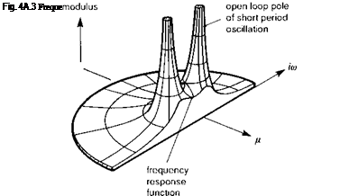
The response vector X is generally complex with a magnitude and phase relative to the input function F. Figure 4A.3 illustrates how the magnitude of the frequency response as a function of frequency can be represented as the value of the so-called transfer function,
when s = iЮ. In Fig. 4A.3 a single oscillatory mode is shown, designated the pitch short period. In practice, for the 6 DoF helicopter model, all eight poles would be present, but the superposition principle also applies to the transfer function. The peaks in the frequency response correspond to the modes of the system (i. e., the roots of the denominator D(s) = 0 in eqn 4A.30) that are set back in either the right-hand side or the left-hand side of the complex plane, depending on whether the eigenvalue real parts are positive (unstable) or negative (stable). The troughs in the frequency response function correspond to the zeros of the transfer function, or the eigenvalues for the case of infinite gain when a feedback loop between input and output is closed (i. e., the roots of the numerator N(s) = 0 in eqn 4A.30). Ultimately, at a high enough frequency, the gain will typically roll-off to zero as the order of D(s) is higher than N(s). The phase between input and output varies across the frequency range, with a series of ramp-like 180° changes as each mode is traversed; for modes in close proximity the picture is more complicated.

For the case when the system modes are widely separated, a useful approximation can sometimes be applied that effectively partitions the system into a series of weakly cou­pled subsystems (Ref. 4A.4). We illustrate the technique by considering the n-dimensional homogeneous system, partitioned into two levels of subsystem, with states x1 and x2, with dimensions I and m, such that n = I + m

_Xi X2

Equation 4A.31 can be expanded into two first-order equations and the eigenvalues can be determined from either of the alternative forms of characteristic equation

Л(*) = XI – A11 – AU(XI – A22)-1 A211 = 0 (4A.32)

Ж*) = XI – A22 – A21 (XI – An)-1 A12 = 0 (4A.33)

Using the expansion of a matrix inverse (Ref. 4A.4), we can write

(XI – A22)-1 = – A-1 (I + XA221 + X2A-22 +—————————– )

We assume that the eigenvalues of the subsystems An |kjJ), kj2), and

A22|k2J 42), …, ї-f} are widely separated in modulus. Specifically, the eigenvalues of Aj j lie within the circle of radius r (r = max|kj!)|), and the eigenvalues of A22 lie without the circle of radius R (R = min|^2;’)|). We have assumed that the eigenvalues of smaller modulus belong to the matrix A jj. The method of weakly coupled systems is based on the hypothesis that the solutions to the characteristic eqn 4A.32 can be approximated by the roots of the first m + J terms and the solution to the characteristic eqn 4A.33 can be approximated by the roots of the last I + J terms, solved separately. It is shown in Ref. 4A.4 that this hypothesis is valid when two conditions are satisfied:

( J ) the eigenvalues form two disjoint sets separated as described above, i. e.,

[r] << J (4A.35)

(2) the coupling terms are small, such that if у and S are the maximum elements of the coupling matrices A 2 and A2 , then

When these weak coupling conditions are satisfied, the eigenvalues of the complete system can be approximated by the two polynomials

f1(*) = 1*1 – Aj J + Aj2 A—J A211 = 0 (4A.37)

f2W =|*I – A221 = 0 (4A.38)

According to eqns4A.37 and4A.38, the larger eigenvalue set is approximated by the roots of A22 and is unaffected by the slower dynamic subsystem AJJ. Conversely, the smaller roots, characterizing the slower dynamic subsystem AJJ, are strongly affected by the behaviour of the faster subsystem A22. In the short term, motion in the slow modes does not develop enough to affect the overall motion, while in the longer term, the faster modes have reached their steady-state values and can be represented by quasisteady effects.

The method has been used extensively earlier in this chapter, but here we provide an illustration by looking more closely at the longitudinal motion of the Puma helicopter in forward flight, given by the homogeneous form of eqn 4A.7, i. e.,

The eigenvalues of the longitudinal subsystem are the classical short period and phugoid modes with numerical values for the J00-knot flight condition given by

Phugoid: kJ>2 = —0.0Ю3 ± 0d76i (4A.40)

Short period: Л3 4 = —L0 ± L30i (4A.4J)

While these modes are clearly well separated in magnitude (r/R = O(0.2)), the form of the dynamic system given by eqn 4A.39 does not lend itself to partitioning as it stands. The phugoid mode is essentially an exchange of potential and kinetic energy, with excursions in forward velocity and vertical velocity, while the short period mode is a rapid incidence

adjustment with only small changes in speed. This classical form of the two longitudinal modes does not always characterize helicopter motion however; earlier in this chapter, it was shown that the approximation breaks down for helicopters with stiff rotors. For articulated rotors, the equations can be recast into more appropriate coordinates to enable an effective partitioning to be achieved. The phugoid mode can be better represented in terms of the forward velocity u and vertical velocity

w0 = w — Ue в (4A.42)

Equation 4A.39 can then be recast in the partitioned form

	u		Xu g cos 0e/Ue	Xw — g cos 0e/Ue Xq — We	u
d	w0		Zu g sin 0e/Ue	Zw — g sin 0e/Ue Zq	w0
dt	w		Zu g sin 0e/Ue	Zw — g sin 0e/Ue Zq + Ue	w
	. q.		Mu 0	— 1 sf S3*	q

(4A.43)

The approximating polynomials for the phugoid and short period modes can then be derived using eqns 4A.37 and 4A.38, namely

Low-modulus phugoid (assuming Zq small):

(xw — UL cos 0^j (ZuMq — Mu (Zq + Ue))

High-modulus short period:

f2(k) = k2 — (Zw + Mq )k + Zw Mq — Mw (Zq + Ue) = 0 (4A.45)

A comparison of the exact and approximate eigenvalues is shown in Table 4A.1, using the derivatives shown in the charts of Appendix 4B. The two different ‘exact’ results are given for the fully coupled longitudinal and lateral equations and the uncoupled longitudinal set. Comparisons are shown for two flight speeds – 100 knots and 140 knots. A first point to note is that the coupling with lateral motion significantly reduces the phugoid damping,

Table 4A.1 Comparison of exact and approximate eigenvalues for longitudinal modes of motion Forward flight speed 100 knots Forward flight speed 140 knots Phugoid Short period Phugoid Short period Exact coupled Exact uncoupled Weakly coupled approximation —0.0103 ± 0.176i —0.0153 ± 0.177i —0.025 ± 0.175i — 1.0 ± 1.30i —0.849 ± 1.17i —0.85 ± 1.47i —0.0006 ± 0.14i —0.0187 ± 0.147i —0.022 ± 0.147i — 1.124 ± 1.693i —0.96 ± 1.583i —0.963 ± 1.873i

particularly at 140 knots where the oscillation is almost neutrally stable. The converse is true for the short period mode. The weakly coupled approximation fares much better at the higher speed and appears to converge towards the exact, uncoupled results. The approximations do not predict the growing loss of phugoid stability as a result of coupling with lateral dynamics, however. The higher the forward speed, the more the helicopter phugoid resembles the fixed – wing phugoid where the approximation works very well for aircraft with strongly positive manoeuvre margins (the constant term in eqn 4A.45 with negative Mw).

The approximations given by eqns 4A.44 and 4A.45 are examples of many that are discussed in Chapter 4 and that serve to provide additional physical insight into complex behaviour at a variety of flight conditions. The importance of the speed stability derivative Mu in the damping and frequency of the phugoid is highlighted by the expressions. For a low-speed fixed-wing aircraft, Mu is typically zero, while the effect of pitching moments due to speed effects dominates the helicopter phugoid. The last term in eqn 4A.45 represents the manoeuvre margin and the approximation breaks down long before instability occurs at positive values of the static stability derivative Mw (Ref. 4A.5).

To complete this appendix we present two additional results from the theory of weakly coupled systems. For cases where the system partitions naturally into three levels

A11	A12	A13
A21	A22	A23
A31	A32	A33

then the approximating polynomials take the form (see Ref. 4A.6)