Sensor Fault Detection Scheme

In order to evaluate the sensor fault detection scheme, primarily only one kind of sensor fault can be considered, that is, a shift in the mean of measurement noise. For fault detection, isolation, and accommodation, extended Kalman filter (EKF) in discrete time domain is mainly used. Sensor fault detection is performed by checking the change in the mean of time series of innovation sequences computed over a window length M (usually M = 20 would suffice). The hypothesis used for fault detection is as follows:

Hq (no fault): b(k) < xl H (fault): b(k) > xl

Here, xl is a threshold obtained from a chi-square table for a confidence probability i = 0.95 (present case) and degree of freedom Ms = M* number of measurement channels. The statistical function b(k) is computed using the following equation:

k

b(k) = Y, nT (j)S~l(MJ) (8.29)

j=k—M+1

Once the hypothesis H1 is satisfied, the next step is to find the source of fault, i. e., the malfunctioning measurement channel. Assuming that there are total “m” channels, the algorithm to isolate the faulty channel is given by

Ho, ch (no fault in “ch” channel): bch(k) < xl, ch Hi, ch (faulty ‘‘ch’’ channel): bch(k) > xl, ch

Here, ‘‘ch’’ is the channel number, which varies from 1 to m and xl ch is a threshold obtained from a chi-square table for a confidence probability i = 0.95 and degree of freedom Ms ch = M — 1. The statistical function bch(k) is computed using the follow­ing equation:

Example 8.5

Realize the sensor fault detection scheme of Figure 8.10 in MATLAB based on the foregoing theory.

Matrices A, B, and G given here [10] can be used for generation of the data:

"—0.033	0.0001	0	—9.81		0.45		1	0	0	0
0.168	—0.3870	260	0	; в =	—5.18	; G =	0	1	0	0
0.005	—0.0064	—0.55	0	—0.91	0	0	1	0
0	0	1	0		0.00		0	0	0	1

Solution

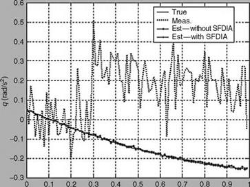
Data simulation is carried out using Equations 8.26 and 8.27 to generate the true and measured states for aircraft longitudinal motion (ExampleSolSW/Example8.5kF). Each element of “Q” is kept at 1.0e — 8, whereas, “R” under normal-sensor operation is kept at diag[0.1296 0.0009 0.0225 0.010]. In the case of SFDIA scheme, the total number of data points simulated is kept at 100 and for AFDIA 2000 data points are simulated. The control input “uc” is kept at a constant value of 8. To first evaluate SFDIA scheme, a fault is introduced in the 3rd channel (i. e., in pitch rate) measurement at the 31st second by adding a constant bias of 0.4°/s to that channel. Figure 8.12 shows the comparison of actual and faulty measurements of pitch rate for 100 data points.

Time (s)

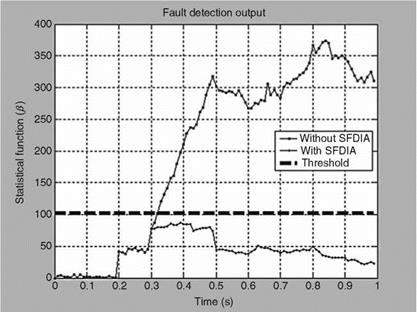
The fault detection is first carried out by comparing the statistical function b(k) with the threshold x2a selected using chi-square table. Threshold is kept at 101.88 for 20DOF and with a confidence level of 0.95. Figure 8.13 shows the comparison of b(k) with the threshold for the entire set of data points. It can be observed from the figure that fault is detected with a delay of four scans (0.04 s). The fault detection automat­ically triggers the isolation algorithm to locate the faulty channel and once the fault is located the accommodation algorithm bypasses the faulty measurements used in the state update of EKF. Figure 8.13 also compares b(k) computed for faulty and reconfigured cases. It is clear that after fault reconfiguration, b(k) never exceeds the threshold value, thereby indicating the proper handling of the faulty channel through the algorithm. The outcome of fault isolation in terms of comparison of the statistical function computed for each measurement channel with the threshold value of 31.4 for 19DOF and with a confidence level of 0.95 was that, except for the third channel, b(k) never exceeded the threshold for the remaining channels, thereby indicating the source of the fault occurrence. b(k) goes below the threshold immediately after the isolation and reconfiguration. Figure 8.14 depicts the innovation sequences along with the theoretical bounds of fSii, where S is the innovation covariance matrix and the term “i” indicates the index of diagonal elements. It can be seen from Figure 8.14 that for the faulty channel (third), the innovation sequence exceeds the bound if not reconfigured, whereas, it is forced to zero after reconfiguration. The estimated states were found to be close to the true states, thereby confirming satisfactory performance of the scheme.

8.8.1
Actuator Fault Detection Scheme

The actuator fault detection scheme is shown in Figure 8.11. The actuator fault can be modeled by multiplying the appropriate component of control vector “B” (Equa­tion 8.26) by the factor of effectiveness. The 50% loss in effectiveness means the faulty value is half of the true value. After the introduction of a fault in some of the components of control vector B, the measurements should be generated using Equations 8.26 and 8.27. The EKF filter should be reformulated as far as the plant model is concerned by augmenting the plant state with the states pertaining to components of B that have to be estimated. The reformulated plant model used in the filter is given by

~a — Aaxa (8-31)

Here, the augmented state xa consists of xa — [ x B ] and the augmented matrix Aa for single control input is given by