Function Catalog

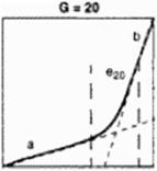
A set of functions Y(X) is suitably defined within the interval 0 < X < I. with end values at X. Y » (0. 0) and (1, 1). see Figure 53. We can imagine a multiplicity of algebraic and other explicit functions Y(X) fulfilling the boundary requirement and. depending on their mathematical struc­ture. allow ing for the control of certain properties especially at the interval ends. Four parameters or less were chosen to describe end slopes (a. bland two additional properties (c^. fG) depending on a function identifier G. The squares shown depict some algebraic curses where the additional parameters describe exponents in the local expansion (G=1), zero curvature without <G=2) or with (G=20) straight ends added, polynomials of fifth order (G=6, quintics) and with square root terms (G=7) allowing curvatures being specified at interval ends. Other numbers for G yield splines, simple Bezier parabolas, trigonometric and exponential functions. For some of them a. b. cq and/or fG do not have to be specified because of simplicity, like G=4 which yields just a straight line. The more recently introduced functions like G=20 gisc smooth connections as well as the limiting cases of curves w ith steps and comers Implementation of these mathematically explicit relations to the computer code allows for using functions plus their first, second and third derivatives. It is obvious that this library of functions is modular and may be extended for special applications, the new functions fit into the system as long as they begin and end at (0.0) and (I, 1). a and b – if needed – describe the slopes and two additional parameters are permitted.

Y = Fq(a, Ь, Є$, 1q, X)

9.2.1 Curves

The next step is the composition of curves by a piecewise scaled use of these functions. Figure

54 illustrates this for an arbitrary set of support points, with slopes prescribed in the supports and curvature or other desired property of each interval determining the choice of function identifiers G. The difference to using spline fits for the given supports is obvious: for the price of having to prescribe the function identifier and up to four parameters for each interval we have a strong con­trol over the curve. The idea is to use this control for a more dedicated prescription of special acrodynamically relevant details of airframe geometry, hoping to minimize the number of opti­mization parameters as well as focusing on problem areas in CFD flow analysis code develop­ment. Numbers serving as names ("keys*’) distinguish between a number of needed curves, the example shows two different curves and their support points. Besides graphs a tabic of input numbers is depicted, illustrating the amount of data required for these curves. Nondimensional function slopes a. b arc calculated from input dimensional slopes s( and s2. as well as the addi­tional parameters Cq, f^ arc found by suitable transformation of c and f. A variation of only sin­gle parameters allows dramatic changes of portions of the curves, observing certain constraints and leaving the rest of the curve unchanged. This is the main objective of this approach, allowing strong control over specific shape variations during optimization and adaptation.

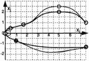Figure 54 Construction of arbitrary, dimensional curves in plane (Xj, Xj) by piecewise use of scaled basic functions. Parameter input list with 2 parameters changed (shaded curves).