Reconfiguration Concept

The technique used is known as pseudo-inverse or control mixer. The dynamics of an unimpaired closed loop system is given by

x = Ax + Buc = Ax + B(—Kx) = (A — BK)x (8.33)

Here, K is the gain matrix and is designed in such a way that eigenvalues of (A — BK) are in the left half of s-plane. The gain K can be computed using MATLAB function ‘‘LQR ()’’ and tuning its parameters by trial-and-error method until it gets the desired response from the system. In the case of the impaired system, the reconfigured closed loop dynamics is given by

x = Ax + Buc = Ax + B(—Kx) = (A — B Ki)x (8.34)

In order to achieve a nearly similar response from the reconfigured impaired system, the RHS of Equation 8.34 should be made equal to RHS of Equation 8.33, i. e.,

A — BK = A — BKi
BK = BKi

The gain matrix for the impaired system can be computed from Equation 8.35

Ki = (B)#BK (8.36)

Here, # is the pseudo-inverse of control vector parameters of B estimated using augmented EKF.

Example 8.6

Realize the actuator fault detection scheme of Figure 8.11 in MATLAB based on the foregoing theory.

The rest of the equations used in augmented EKF are the same as those used in the scheme of Example 8.5 (ExampleSolSW/Example8.6AFDIA). The estimated value of the control vector is subsequently used for reconfiguration of impaired aircraft. For evaluation of this scheme, the fault in the actuator is introduced at the 100th iteration by changing the third element of control input vector B from its actual value of —0.91 to —0.45, i. e., nearly 50% loss in effectiveness. Figure 8.15 shows the states correspond­ing to longitudinal motion of the aircraft for unimpaired and impaired configurations. It can be seen that the states for both the configurations are comparable up to the first 5 s and thereafter a clear difference in magnitude of state of the values can be seen. The measurements are generated using the state of impaired aircraft and subsequently used to recursively estimate the elements of input control matrix B using the scheme. For the estimation of B as an augmented state with the state pertaining to longitudinal motion, EKF is used with its initial state kept at zero and accordingly state initial error covariance is computed. The tuning parameters such as Q and R are assumed to be known precisely. Figure 8.16 illustrates the estimated values of B compared with true values. B(1) converges to the true value as the number of data increases. In the case of the faulty element B(3), initially the estimated value starts from zero and then converges to true value and when the fault occurs it slowly tries to converge to the faulty value. These estimated values are subsequently used in control reconfiguration to make the performance of the impaired aircraft close to an unimpaired one. Under the scheme, first the response of the unimpaired aircraft with state feedback and without control input (i. e., uc = 0) is realized by designing the feedback gain matrix K (Equation 8.36), using the LQR method (in MATLAB). During the analysis, it is found that with feedback gain K = [0.0886 0.0048 —0.8906 —2.1274], and closed loop or controlled response of the longitudinal state tends to zero as required. The parameters, such as feedback gain K for

Time (s) Time (s)

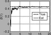
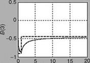
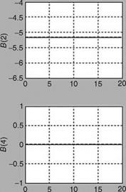
FIGURE 8.16 Comparison of true and estimated elements of control input matrix ‘‘B’’.

unimpaired aircraft, estimated B along with true B and A, are used to reconfigure the feedback gain for impaired aircraft. Figure 8.17 compares the closed loop response of unimpaired, impaired without reconfiguration, and reconfigured impaired aircraft. It is observed from the plots that the response of the reconfigured state converges to that of the unimpaired one, thereby indicating reconfiguration of the faulty system. However, much