System Identification and Parameter Estimation

9.1 INTRODUCTION

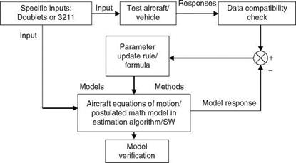
The system identification and parameter-estimation process (SIPEP), one of the important approaches to mathematical modeling, provides a powerful tool for sys­tematic analysis and eventual optimization of industrial processes, thereby reducing losses and saving the cost of production. The SIPEP is a fairly mature technology and can be considered as a data-dependent model building process. In aerospace applications it can be used to great advantage to aid the iterative control-law design/flight simulation cycles as well as in certification of atmospheric vehicles. System identification (SID) refers to the determination of an adequate mathematical model structure based on the physics of the problem and analysis of available data using some optimization criterion to minimize the sum of the squares of errors between the responses of the postulated mathematical model and the real system. The computational procedure is generally iterative and requires engineering judg­ment and use of objective model selection criteria [1]. Parameter estimation is also employed in the SID procedure. Parameter estimation is regarded as a special case of SID procedure and also of Kalman filtering methods. Parameter estimation refers to explicit determination of numerical values of unknown parameters of the postulated state-space mathematical model, or any type of the model. The basic principles are the same as in SID but in many cases the model structure selection procedure may not be needed due to the availability and use of well-defined structure from the physics of the system (Chapters 3 through 5), e. g., aircraft parameter estimation. The SIPEP for a flight vehicle is illustrated in Figure 9.1.

The SIPEP utilizes techniques and principles from several established branches of mathematics, science, and engineering: (1) general and applied mathematics for definition of mathematical models; (2) statistical and probability theory for inter­pretation of results and definition of cost functions/criteria (Appendix B, [2]); (3) optimization methods and theory of model reduction for optimal solutions; (4) numerical techniques for solution of differential equations and matrix inversion; (5) system and control theory for state-space and transfer function modeling (Appen­dix C, Chapter 2); (6) signal processing for fast Fourier transform (FFT), spectral density evaluation, and filtering of signals (Appendix C); (7) linear algebra for vector/matrix and related theories (Appendix B); and (8) information theory for interpretation of results and definition of criteria. More often the configuration of the SIPEP used for a particular application is governed by the state-of-the-art

Maneuvers Measurements FIGURE 9.1 System identification/parameter estimation procedure.

development in the above areas. Therefore, a continual upgradation may be required to extract benefits from these supportive disciplines. The development of SIPEP takes place at various stages and levels as an independent R&D effort. In initial stages a considerable trial and error approach is used with simulated and real data to arrive at the most appropriate methods. No single method is perfectly suitable for all kinds of problems studied/encountered.

Some typical major developments have been in the following areas (some examples are presented in this chapter): (1) implementation and use of time-series analysis methods for modeling of dynamic systems (e. g., modeling of human operator’s dynamics in a compensatory control task in a flight research simulator) [3]; (2) enhancement of output error method (OEM) based algorithm for parameter estimation of inherently unstable/augmented control system (e. g., unstable-fly­by-wire (FBW) aircraft), development of analysis techniques for parameter estima­tion of unstable dynamic systems [1]; (3) development of factorization-based extended Kalman filtering programs for flight path reconstruction and data compati­bility checking of flight test data [4]; (4) development of serial/parallel schemes for implementation of genetic algorithms (GAs) with the purpose of using for parameter estimation [1]; (5) development of new architectures for parameter estimation using recurrent neural networks (RNNs) and fast algorithms for training of feed forward neural networks (FFNNs) [1]; and (6) development of a filter-error-based program for parameter estimation of stable/unstable systems with data corrupted by colored noise (turbulence) [5].

The expansive scope of SIPEP encompasses other related areas: (1) Online real­time system identification and parameter-estimation technology poses the challenging task of arriving at the synergism of robust, accurate, and stable computational algo­rithms, efficient programming, choice of suitable cost-effective and yet fast computers (serial or parallel), and thorough validation under realistic test conditions to guarantee overall trouble-free operation in real-life practical environment. Certain time-varying properties of systems can be tracked by using online real-time system identification – cum-parameter estimation for use in adaptive control [6]; (2) Incorporation of ‘‘soft computing’’ into the traditional/conventional SIPEP. Here, ANNs, fuzzy logic-based concepts, and GAs can be effectively used to develop expert system-based SIPEP; (3) Use of SID procedures for near real-time determination of gain – and phase-margins of an FBY aircraft during flight testing exercises; (4) Use of GPS receiver signals in conjunction with the existing sensor-measurement data to improve the accuracy of estimates, e. g., flight path reconstruction using GPS signals, air data calibration exercises [7]; (5) Multisensor data fusion technology that utilizes Kalman – and information-based filtering algorithms for kinematic fusion of the state vector from individual sensor updates. SIPEP can also play a significant role in this field [8].

Several criteria are used to judge the ‘‘goodness’’ of the estimator/estimates: Cramer-Rao bounds (CRBs) of the estimates, correlation coefficients among the estimates, determinant of the covariance matrix of the residuals, plausibility of the estimates based on physical understanding of the dynamic system, comparison of the estimates with those of nearly similar systems or estimates independently obtained by other methods (analytical or other parameter-estimation methods), and model predictive capability. The time-history match is a necessary but not sufficient condition. It is quite possible that the response match would be good but some parameters could be unrealistic due to (1) deficient model used for the estimation and (2) insufficient excitation of some modes of the system. One way to circumvent this problem is to add a priori information about the parameter in question, or to add a constraint in the cost function, with a proper sign (constraint) on the parameter. One more approach is to fix such parameters at some a priori value, which could have been determined by some other means or available independently from another source from the system. A simple and commonly followed procedure [9] for SIPEP (see Figure 9.1) has the following steps:

• Data gathering/recording from the planned experiments on the process/ plant/system; this presupposes proper experiment planning, design of input signal, test conditions, etc.

• Data preprocessing to remove spikes/extraneous noise, kinematic consist­ency checking for aircraft parameter estimation

• Postulation of appropriate model structure (Chapters 2 and 5)

• Selection of criteria for model structure determination—usually data depen­dent (Chapter 6 of Ref. [1])

• Estimation of parameters of the postulated model using suitable parameter – estimation method [1]

• Performance evaluation of the identified model/parameters using goodness – of-fit criteria

• Model validation across the validation data sets from the same experiment

• Revisiting the postulated model and refining the model if needed; may be improving models with additional data

• Interpretation of the results and specification of the confidence in the derived results from SIPEP

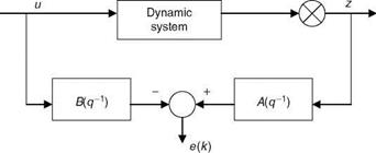
Since the data u(k) and z(k) are available from the experiments, the above equations can be put in the form

z = Hb + e (9.4)

Here, z = {z(n + 1), z(n + 2),…, z(n + N)}T with

	—z(n)	—z(1)	u(n)	u(1)’
H =	—z(n + 1)	—z(2)	u(n + 1)	u(2)	(9.5)
	—z(N + n — 1) ••	• – z(n)	u(N + n — 1)	.. u(N)

N is equal to the number of the data used. For example, with n = 3 and m = 1, we have

e(k) = z(k) + az(k — 1) + Я2 z(k — 2) + a3z(k — 3) — b0u(k) — bu(k — 1) (9.6)

and so on, thereby yielding, in collective form, Equation 9.4, with appropriate equivalence. Using the LS method, we get the estimates of the parameters as

b = {fib…, fin. fib…, bm} = (HTH)—1 HTz (9.7)

The coefficients of time-series models can be estimated using the SID toolbox of MATLAB. An example of human operator modeling using the time-series approach is given in Chapter 10. The covariance matrix of parameter-estimation error is given as

cov(b — b) « s2(HTH)—1 (9.8)

Here, sr2 is the estimation-residual variance.

In aircraft parameter estimation, a general form of the model to be identified occurs as

y(t) = bo + btxt(f) H———— E bn—1xn—1(t) + e(t) (9.9)

dynamic system; in fact, some intermediate steps might be required to compute y from x. This is true for aircraft parameter estimation, and the intermediate compu­tations will involve all the known constants and variables like xt and y. It is necessary to determine the parameters that should be retained in the model and estimated. This problem is handled using model order determination criteria and the LS method for parameter estimation. In aircraft parameter estimation, often y(t) represents the aerodynamic coefficients (Chapter 4) and b the aerodynamic derivatives.