Fuselage aerodynamic characteristics

Chapter 3 developed a generalized form for the aerodynamic forces and moments acting on the fuselage; Table 4B.4 presents a set of values of force and moment coefficients, giving one-dimensional, piecewise linear variations with incidence and sideslip. These values have been found to reflect the characteristics of a wide range of fuselage shapes; they are used in Helisim to represent the large angle approximations.

Small angle approximations (-20° < (af, вf) < 20°) for the fuselage aerodynamics of the Lynx, Bo105 and Puma helicopters, based on wind tunnel measurements, are given in eqns 4B.1 – 4B.15. The forces and moments (in N, N/rad, N m, etc.) are given as functions of incidence and sideslip at a speed of 30.48 m/s (100 ft/s). The increased order of the polynomial approximations for the Bo105 and Puma is based on more extensive curve fitting applied to the wind tunnel test data. The small angle approximations should be fared into the large angle piecewise forms.

Lynx

,0 = -1112.06 + 3113.75 a2f	(4B.1)
Xf100 = —8896.44 в f	(4B.2)
Zf100 = —4225.81 a f	(4B.3)
Mf100 = 10 168.65 a f	(4B.4)
Nf100 = -10168.65 ef	(4B.5)

Table 4B.4 Generalized fuselage aerodynamic coefficients a f — 180 — 160 —90 —30 0 20 90 160 180 Cxf 0.1 0.08 0.0 —0.07 —0.08 —0.07 0.0 0.08 0.1 a f — 180 — 160 — 120 —60 —20 0 20 60 120 160 180 Czf 0.0 0.15 1.3 1.3 0.15 0.0 —0.15 —1.3 —1.3 —0.15 0.0 a f —205 — 160 — 130 —60 —25 25 60 130 155 200 Cmf 0.02 —0.03 0.1 0.1 —0.04 0.02 —0.1 —0.1 0.02 —0.03 в f —90 —70 —25 0 25 70 90 Cnfa —0.1 —0.1 0.005 0.0 —0.005 0.1 0.1 в f —90 —60 0 60 90 Cnfb —0.1 —0.1 0.0 0.1 0.1

Bo105

Xf loo = -580.6 – 454.0 af + 6.2 a2 + 4648.9 a3 (4B.6)

Yfloo = -6.9 – 2399.0 вf – 1.7 в] + 12.7 в] (4B.7)

Zf100 = -51.1 – 1202.0 af + 1515.7 a2f – 604.2a3 (4B.8)

Mf100 = -1191.8 + 12752.0 af + 8201.3 a2f – 5796.7 a3 (4B.9)

Nf100 = -10028.0 ву (4B.10)

Puma

Xf100 = -822.9 + 44.5 a f + 911.9 a2f + 1663.6 a3 (4B.11)

Yf100 = -11 672.0 в f (4B.12)

Zf100 = -458.2 – 5693.7 af + 2077.3 a2f – 3958.9 af (4B.13)

Mf100 = -1065.7 + 8745.0af + 12473.5af – 10033.0af (4B.14)

Nf100 = -24 269.2 вf + 97 619.0 в} (4B.15)

Empennage aerodynamic characteristics

Following the convention and notation used in Chapter 3, small angle approximations (-20° < (atp, вfn) < 20°) for the vertical tailplane and horizontal fin (normal) aerodynamic force coefficients are given by the following equations. As for the fuselage forces, the Puma approximations have been curve fitted to greater fidelity over the range of small incidence and sideslip angles.

Lynx

Cztp = -3.5 atp (4B.16)

Cyfn = -3.5 вп (4B.17)

Bo105

Cztp = -3.262 atp (4B.18)

Cyfn = -2.704 вп (4B.19)

Puma

Cztp = -3.7 (atp – 3.92ajP) (4B.20)

4B.2 Stability and control derivatives

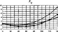
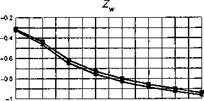
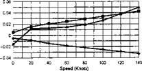
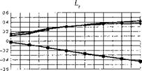
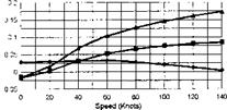
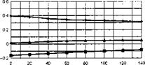
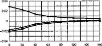
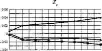
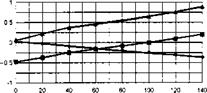
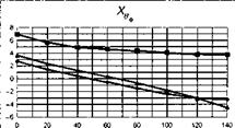
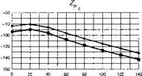
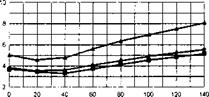
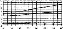
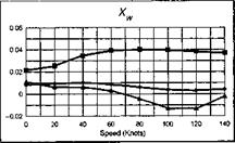
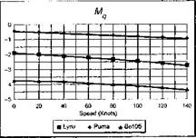
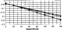
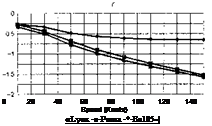
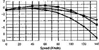
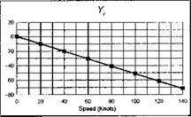
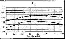
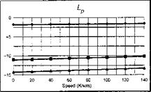
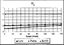
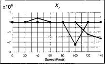
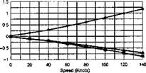
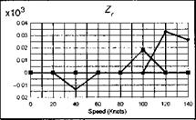
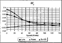
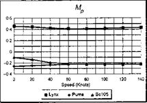
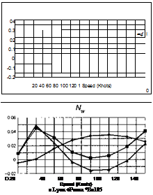
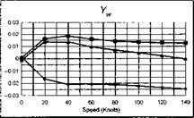
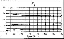
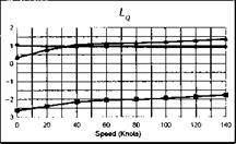
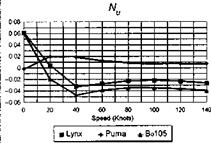
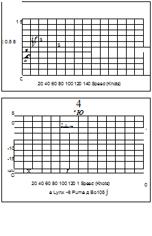
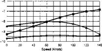
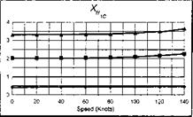
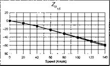
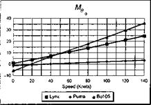
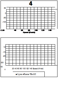
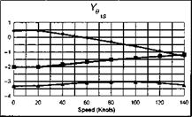
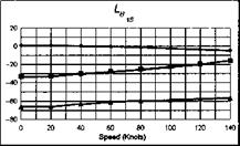
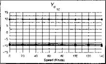
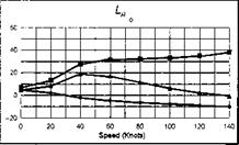
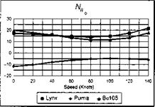
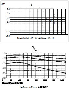
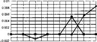
The stability and control derivatives predicted by Helisim for the three subject helicopters are shown in Figs 4B.7-4B.13 as functions of forward speed. The flight conditions correspond to sea level (p = 1.227 kg/m3) with zero sideslip and turn rate, from hover to 140 knots. Figures 4B.7 and 4B.8 show the direct longitudinal and lateral derivatives respectively. Figures 4B.9 and 4B.10 show the lateral to longitudinal, and longitudinal to lateral, coupling derivatives respectively. Figures 4B.11 and 4B.12 illustrate the longitudinal and lateral main rotor control derivatives, and Fig. 4B.13 shows the tail rotor control derivatives. As an aid to interpreting the derivative charts, the following points should be noted:

(1) The force derivatives are normalized by aircraft mass, and the moment derivatives are normalized by the moments of inertia.

(2) For the moment derivatives, pre-multiplication by the inertia matrix has been carried out so that the derivatives shown include the effects of the product of inertia Ixz (see eqns 4.47-4.51).

(3) The derivative units are as follows:

force/translational velocity	e. g. Xu	1/s
force/angular velocity	e-g – Xq	m/s. rad
moment/translational velocity	e. g. Mu	rad/s. m
moment/angular velocity	e. g. Mq	1/s
force/control	e. g. X00	m/s2 rad
moment/control	e. g. M0o	1/s2

(4) the force/angular velocity derivatives, as shown in the figures, include the trim velocities, e. g.,

7 = 7 U

— Zv q + ‘-d e

*u -0.01 -0.02! -0.03 -0.04 -0.05 -0.06 3 I 0 20 40 60 80 100 120 1 Speed (Knots) 0.05 0 z u ; &V -0.05 -0.1 -0.15 -0.2 г** ~r. у / V -0.25 0 20 40 60 80 100 120 140 Speed (Knots) r 0.12 r M u s. 0.08 0.06 s. 4 0.04* 0.02 N c=. 0 0 20 40 60 80 100 120 140 Speed (Knots) ;*Lynx ♦Puma *Bo105[

Speed (Knots)

60 40 20 -20 20 40 60 80 100 120 140 Speed (Knots)

О 20 40 60 80 100 120 140 Speed (Knots)

[ ■ Lynx ♦ Puma ♦ Bo105 |

0 20 40 60 80 100 120 140 Speed (Knots)

«Lynx ♦Puma -*-Bo105

Speed (Knots)

Speed (Knots)

0 20 40 60 80 100 120 140 Speed (Knots)

x106 M Г 0.8 0.6 0.4 0.2 • у Л / V t r / j V T V . ( -0.2 ( ** 0 20 40 60 80 100 120 1 Speed (Knots) И Lynx *-Puma *Bo105 |

: oo4 : 0 021 і o і : -0.02 Yu -0 04 20 40 60 80 100 120 140 Speed (Knots) Lu ■ X ‘ ‘ ‘ і „ . і 0 —— — 0 20 40 60 80 100 120 140 Speed (Knots)

Speed (Knots) *Lynx – e-Puma *-Bo105

Speed (Knots)

Speed (Knots)

60 40 4 IS ‘ 20 0 c zn 0 20 40 60 60 100 120 1 Speed (Knots) j a Lynx e-Puma *Bo105 |

5 04 % IS -10 c 20 40 60 80 100 120 140 Speed (Knots) | * Lynx ♦Puma *Bo105

x103 0 01 — — <0 C T —– -0 01 -0.02 -0 03 C V ) ■ ■> / ■N I r 20 40 60 80 100 Speed (Knots) 120 140
Speed (Knot3)
Mn
x1Cr
Speed (Knots) ■ Lynx ♦Puma *Bo105
Speed (Knots) I Lynx ♦ Puma * Bo105

Appendix 4C the Trim Orientation Problem

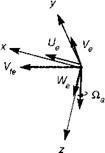
In this section we derive the relationship between the flight trim parameters and the velocities in the fuselage axes system, for use earlier in the chapter. Figure 4C. 1 shows the trim velocity vector Vfe of the aircraft with positive components along the fuselage axes directions x, y and z given by Ue, Ve and We respectively, where subscript e denotes equilibrium.

The trim condition is defined in terms of the trim velocity Vfe, the flight path angle Yfe, the sideslip angle Д. and the angular velocity about the vertical axis Qae. The latter plays no part in the translational velocity derivations. The incidence and sideslip angles are defined as

&e = tan-1 ^ W^ (4C.1)

Pe = sin-1 ((4C.2)

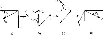
The sequence of discrete orientations required to derive the fuselage velocities in terms of the trim variables is shown below in Fig. 4C.2.

The axes are first rotated about the horizontal y-axis through the flight path angle. Next, the axes are rotated through the track angle, positive to port (corresponding to a positive sideslip angle) giving the orientation of the horizontal velocity component relative to the projected aircraft axes. The final two rotations about the Euler pitch and roll angles bring the axes into alignment with the aircraft axes as defined in Chapter 3, Section 3A.1.

Fig. 4C.1 Flight velocity vector relative to the fuselage axes in trim

Fig. 4C.2 Sequence of orientations from velocity vector to fuselage axes in trim: (a) rotation to horizontal through flight path angle yf; (b) rotation through track angle x; (c) rotation through Euler pitch angle 0; (d) rotation through Euler roll angle Ф

The trim velocity components in the fuselage-fixed axis system may then be written as
Ue = Vfe (cos @e cos Yfe cos xe — sin @e sin ye)

(4C.3)

Ve = Vfe (cos Фє cos Yfe sin xe + sin Фє (sin @e cos Yfe cos xe + cos @e sin Yfe))

(4C.4)

We = Vfe (—sin Фє cos Yfe sin xe + cos Фє (sin Qe cos Yfe cos xe + cos @e sin y^

(4C.5)

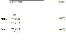
The track angle is related to the sideslip angle through eqn 4C.4 above. The track angle is then given by the solution of a quadratic, i. e.,

sin

where

and the к coefficients are

kX1 = sin Фє sin Qe cos Yfe	(4C.9)
kX2 = cos Фє cos Yfe	(4C.10)
kX3 = sin ee — sin Фє cos Qe sin Yfe	(4C.11)

Only one of the solutions of eqn 4C.6 will be physically valid in a particular case.

Finally, the relationship between the fuselage angular velocities and the trim vertical rotation rate can be easily derived using the same transformation as for the gravitational forces. Hence,

Pe = -&ae sin Qe (4C.12)

Qe = &ae cos Qe sin Фе (4C.13)

Re = Q, ae cos Qe cos Фє (4C.14)

Note that for conventional level turns, the roll rate p is small and the pitch and yaw rates are the dominant components, with the ratio between the two dependent upon the trim bank angle. In trim at high climb or descent rates the pitch angle can be significantly different from zero, increasing the roll rate in the turn manoeuvre.

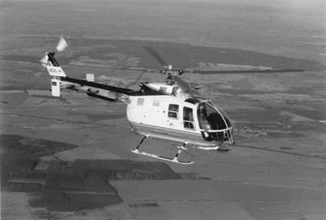
The German DLR variable stability (fly-by-wire/light) Bo105 S3
(Photograph courtesy of DLR Braunschweig)