Hover and Vertical Flight

The formula relating thrust and power in vertical flight, according to blade element theory, was derived in Equation 3.54. The power required is the sum of induced power, related to blade lift, and profile power, related to blade drag. Converting to dimensional terms the equation is:

1 ,

P = ki(VC + Vi)T + 8 CD0MbVT (7.1)

where in the induced term, using momentum theory as in Equation 2.28, one may write:

If in Equation 7.1 the thrust is expressed in N, velocities in m/s, area in m2 and air density in kg/m3, the power is then in W or, when divided by 1000, in kW. Using imperial units, thrust in lb, velocities in ft/sec, area in ft2 and density in slugs/ft3 lead to a power in lb ft/sec or, on dividing by 550, to HP.

To make a performance assessment, Equation 7.1 is used to calculate separately the power requirements of main and tail rotors. For the latter, VC disappears and the level of thrust needed is such as to balance the main rotor torque in hover; this requires an evaluation of hover trim, based on the simple equation:

T • / = Q (7.3)

where Q is the main rotor torque and / is the moment arm from the tail rotor shaft perpendicular to the main rotor shaft. The tail rotor power may be 10-15% of main rotor power. To these two are added allowances for transmission loss and auxiliary drives, perhaps a further 5%. This leads to a total power requirement, Preq say, at the main shaft, for a nominated level of main rotor thrust or vehicle weight. The power available, Pav say, is ascertained from engine data, debited for installation loss. Comparing the two powers determines the weight capability in hover, out of ground effect (OGE), under given ambient conditions. The corresponding capability in ground effect (IGE) can be deduced using a semi-empirical relationship such as Equation 2.64. The aircraft ceiling in vertical flight is obtained by matching Preq and Pav for nominated weights and atmospheric conditions.

kiVc, ki /V2, 2T ~ + 2 V Vc + ГА

VC(2—ki) + kiJ VC + 4V0

In order to understand the sensitivity of power in climb to the climb rate, we recall Equation 2.27:

from which we obtain, after partial differentiation with respect to Vc:

where the overbar is used, as in Chapter 2, to denote normalization with respect to V0 and the derivative is related to small increments in power and climb rate.

If this argument is examined in reverse, we have an equation which relates the climb rate achievable for a given excess of power.

Equation 7.7 now becomes:

climb rate factor

where the thrust is assumed to be equal to the aircraft weight in an equilibrium state. The kD factor is applied to the thrust to take account of the fuselage download increased in the climb.

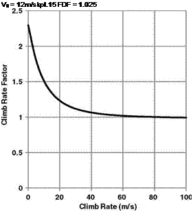Taking kj to be 1.15 and kD to be 1.025, the term in braces in Equation 7.8 is plotted in Figure 7.2.

As the climb rate increases, the climb rate factor term drops from a value of approximately 2 in the hover to approximately 1 at a high climb rate. This is because, as the helicopter climbs away from hover, the climb causes a fall in the value of downwash, saving power which will contribute to that available from the engine(s). As the climb rate increases, the downwash will reduce to a very small value so this beneficial effect is lost and the engine power surplus is all that is available to generate a climb velocity. The two-to-one variation in factor between a zero climb rate and a high climb rate (say 6000 ft/min) is typical. Stepniewski and Keys (Vol. II, p. 55) suggest a linear variation between the two extremes. It should be borne in mind, however, that at low rates of either climb or descent, vertical movements of the tip vortices relative to the disc plane are liable to change the power relationships in ways which cannot be reflected by momentum theory and which are such that the power relative to that in hover is actually decreased initially in climb and increased initially in descent. These effects, which have been pointed out by Prouty [1], were mentioned in Chapter 2. Obviously in such situations Equation 7.4 and the deductions from it do not apply.