Panel Method

7.1 Introduction

Panel method is a numerical technique to solve flow past bodies by replacing the body with mathematical models; consisting of source or vortex panels. Essentially the surface of body to be studied will be represented by panels consisting of sources and free vortices. These are referred to as source panel and vortex panel methods, respectively. If the body is a lift generating geometry, such as an aircraft wing, vortex panel method will be appropriate for solving the flow past, since the lift generated is a function of the circulation or the vorticity around the wing. If the body is a nonlifting structure such as a pillar of a river bridge, the source panel method might be employed for solving the flow past that.

7.2 Source Panel Method

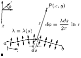
Consider the source sheet of finite length along the ^-direction and extending to infinity in the direction normal to s, as shown in Figure 7.1.

The source strength per unit length along s-direction of the panel, shown in Figure 7.1, is X = X(s). Also, the small length segment ds is treated as a distinct source of strength X ds.

Let us consider a point P as shown in Figure 7.1. The small segment of the source sheet of strength X ds induces an infinitesimally small velocity potential dф at point P. That is:

X ds

= —– ln r.

2n

The complete velocity potential at point P, due to source sheet from a to b, is given by:

In general, the source strength X(s) can change from positive (+ve) to negative (—ve) along the source sheet. That is, the ‘source’ sheet can be a combination of line sources and line sinks.

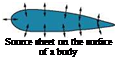
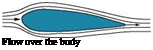
Next, let us consider a given body of arbitrary shape shown in Figure 7.2.

Let us assume that the body surface is covered with a source sheet, as shown in Figure 7.2(a), where the strength of the source X (s) varies in such a manner that the combined action of the uniform flow and the source sheet makes the aerofoil surface and streamlines of the flow, as shown in Figure 7.2(b).

Theoretical Aerodynamics, First Edition. Ethirajan Rathakrishnan.

© 2013 John Wiley & Sons Singapore Pte. Ltd. Published 2013 by John Wiley & Sons Singapore Pte. Ltd.

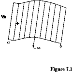Uniform

flow

Figure 7.2 An arbitrary body (a) covered with source sheet, (b) the flow past it.

The problem now becomes that of finding appropriate distribution of k(y), over the surface of the body.

The solution to this problem is carried out numerically, as follows:

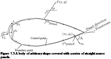
• Approximate the source sheet by a series of straight panels, as shown in Figure 7.3.

• Let the source strength k(y) per unit length be constant over a given general panel, but allow it to vary

from one panel to another. That is, for n panels the source strengths are k, k2, k3,………. , kn.

• The main objective of the panel technique is to solve for the unknowns kj, j = 1 to n, such that the body surface becomes a stream surface of the flow.

•

This boundary condition is imposed numerically by defining the mid-point of each panel to be a control point and by determining the kjs such that the normal component of the flow velocity is zero at each point.

Let P be a point at (x, y) in the flow, and let rpj be the distance from any point on the /h panel to point P, as shown in Figure 7.3. The velocity at P due to the /h panel, Афj, is:

Афі = 2П Iln rPjdsj,

where the source strength Xj is constant over the jth panel, and the integration is over the jth panel only.

The velocity potential at point P due to all the panels can be obtained by taking the summation of the above equation over all the panels. That is:

ф(р) = ^ Аф = ^2 2n Iln rpjds

j=i

where the distance:

rPj = J(x – xj)2 + (y – yj)2,

where (xj, yj) are the coordinates along the surface of the jth panel.

Since P is just an arbitrary point in the flow, it can be taken at anywhere in the flow including the surface of the body, which can be regarded as a stream surface (essentially the stagnation stream surface). Let P be at the control point of the ith panel. Let the coordinates of this control point be given by (x;, y;), as shown in Figure 7.3. Then:

(7.1)

where

rij = J (xi – xj)2 + (y; – yj)2.

Equation (7.1) is physically the contribution of all the panels to the potential at the control point on the ith panel.

The boundary condition is at the control points on the panels and the normal component of flow velocity is zero. Let n be the unit vector normal to the ith panel, directed out of the body.

The slope of the ith panel is (dy/dx);. The normal component of velocity with respect to the ith panel is:

V^,n V(X> ‘ ni V(X> cos Pi,

where в; is the angle between VOT and n;. Note that Vai, n is positive (+ve) when directed away from the body.

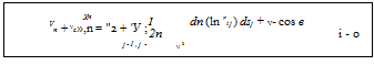
The normal component of velocity induced at (x;, y;) by the source panel, from Equation (7.1), is:

When the differentiation in Equation (7.2) is carried out, rij appears in the denominator. Therefore, a singular point arises on the ith panel because at the control point of the panel, j = i and rtj = 0. It can be

shown that when j – i, the contribution to the derivative is X/2. Therefore:

where Xi/2 is the normal velocity induced at the ith control point by the ith panel itself.

The normal component of flow velocity is the sum of the normal components of freestream velocity V—,n and velocity due to the source panel Vn. The boundary condition states that:

V _i_ V — 0

Therefore, the sum of Equation (7.3) and V—,n results in:

(7.4)

This is the heart of source panel method. The values of the integral in Equation (7.4) depend simply on the panel geometry, which are not the properties of the flow.

Let I-j be the value of this integral when the control point is on the ith panel and the integral is over the jth panel. Then, Equation (7.4) can be written as:

This is a linear algebraic equation with n unknowns Л1, X2, ………… , Xn. It represents the flow boundary

condition evaluated at the control point of the ith panel.

Now let us apply the boundary condition to the control points of all the panels, that is, in Equation (7.5), let i — 1, 2, 3, …., n. The results will be a system of n linear algebraic equations with n unknowns (X1, X2, , Xn), which can be solved simultaneously by conventional numerical methods:

• After solving the system of equations represented by Equation (7.5) with i — 1, 2, 3, …., n, we have the distribution source panel strength which, in an approximate fashion, causes the body surface to be a streamline of the flow.

• This approximation can be made more accurate by increasing the number of panels, hence more closely representing the source sheet of continuously varying strength X (s).