The Vortex Panel Method

This method is analogous to the source panel method studied earlier. The source panel method is useful only for nonlifting cases since a source has zero circulation associated with it. But vortices have circu­lation, and hence vortex panels can be used for lifting cases. It is once again essential to note that the vortices distributed on the panels of this numerical method are essentially free vortices. Therefore, as in the case of source panel method, this method is also based on a fundamental solution of the Laplace equation. Thus this method is valid only for potential flows which are incompressible.

7.3.1 Application of Vortex Panel Method

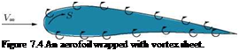
Consider the surface of an aerofoil wrapped with vortex sheet, as shown in Figure 7.4.

We wish to find the vortex distribution y (s) such that the body surface becomes a streamline of the flow. There exists no closed-form analytical solution for y(s); rather, the solution must be obtained numerically. This is the purpose of the vortex panel method.

The procedure for obtaining solution using vortex panel method is the following: [10]

• The mid-point of each panel is a control point at which the boundary condition is applied; that is, at each control point, the normal component of flow velocity is zero.

Let P be a point located at (x, y) in the flow, and let rpj be the distance from any point on the jth panel to P. The radial distance rPj makes an angle 0pj with respect to x-axis. The velocity potential induced at P due to the jth panel [Equation (2.42)] is:

=~2L jj^j

The component of velocity normal to the ith panel is given by:

VX, n VX cos fti.

The normal component of velocity induced at (xi, yi) by the vortex panels is:

d

Vn – dn ^ *>]. (7Л3)

From Equations (7.11) and (7.13), we get the normal component of velocity induced as:

By the boundary conditions, at the control point of the ith, we have:

Vix>,n + Vn — ^

that is:

(7.16)

This equation is the crux of the vortex panel method. The values of the integrals in Equation (7.16) depend simply on the panel geometry; they are properties of the flow.

Let Jj be the value of this integral when the control point is on the ith panel. Now, Equation (7.16) can be written as:

n

Vx cos в – у jjj — 0. (7.17)

j—1

Equation (7.17) is a linear algebraic equation with n unknowns, y,yi, y3, …., yn. It represents the flow boundary conditions evaluated at the control point of the jth panel. If Equation (7.13) is applied to the control points of all the panels, we obtain a system of n linear equations with n unknowns.

The discussion so far has been similar to that of the source panel method. For source panel method, the n equations for the n unknown source strength are routinely solved, giving the flow over a nonlifting body.

For a lifting body with vortex panels, in addition to the n equations given by Equation (7.17) applied at all the panels, we must also ensure that the Kutta condition is satisfied. This can be done in many ways. For example, consider the trailing edge of an aerofoil, as shown in Figure 7.5, illustrating the details of vortex panel distribution at the trailing edge.

Note that the length of each panel can be different, their length and distribution over the body is at our discretion. Let the two panels at the trailing edge be very small. The Kutta condition is applied at the trailing edge and is given by:

Y (te) = 0.

To approximate this numerically, if points i and (i — 1) are close enough to the trailing edge, we can write:

Yi = Yi— 1. (7.18)

such that the strength of the two vortex panels i and (i — 1) exactly cancel at the point where they touch at the trailing edge. Thus, the Kutta condition demands that Equation (7.18) must be satisfied.

Note that Equation (7.17) is evaluated at all the panels and Equation (7.18) constitutes an over­determined system of n unknowns with (n + 1) equations. Therefore, to obtain a determined system, Equation (7.17) is evaluated at one of the control points. That is, we choose to ignore one of the control points, and evaluate Equation (7.17) at the other (n — 1) control points. This, on combination with Equation (7.18), gives n linear algebraic equations with n unknowns.

At this state, conceptually we have obtained Yi, Y2, Y3,……… ,Yn which make the body surface a stream­

line of the flow and which also satisfy the Kutta condition. In turn, the flow velocity tangential to the
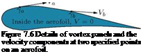
surface can be obtained directly from y. To see this more clearly, consider the aerofoil shown in Figure 7.6.
The velocity just inside the vortex sheet on the surface is zero. This corresponds to u2 = 0. Hence:

Y = U1 — U2 = U1 — 0 = U1.

Therefore, the local velocities tangential to the aerofoil surface are equal to the local values of Y. In turn the local pressure distribution can be obtained from Bernoulli’s equation. The total circulation around the aerofoil is:

n

Г = £) Yjj. (7.19)

j=1

Flow

Hence, the lift per unit span is: