Interpolation Errors in Wave Number Space

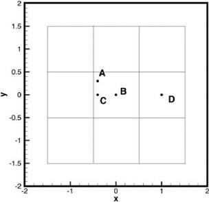
An interpolation stencil may be regular or irregular depending on the configuration of the stencil relative to the coordinate system used for the computation. Generally speaking, interpolation error is small compared with extrapolation error. Figure

13.6 shows a 16-point irregular interpolation stencil. For reference purposes, the coordinates of the interpolation points of this stencil are as follows:

(-0.70,1.72) (0.34,1.58) (1.24, 1.14) (-1.62, 0.72) (-0.38, 0.79) (0.64, 0.60) (-1.02, 0.08) (0.18, -0.20) (1.58, 0.06) (-1.24, -0.56) (-0.38, -0.92) (0.80.-0.78) (-1.56, -1.40) (-0.26, -1.68) (0.66, -1.52) (1.64, -1.16)

The points to be interpolated are as follows:

A (-0.40, 0.30)

B (0.00, 0.00)

C (-0.40, 0.00)

D (1.00,0.00)

Figure 13.7 shows a 16-point regular stencil in the form of a square. Interpolation error analysis for the 4 points A, B, C, and D shown in both Figures 13.6 and 13.7 have been carried out. The finding is that the errors for points A, B, and C are very similar. For this reason, only the interpolation errors of A and D will be discussed. It is useful to consider point A as typical of all the points located around the center of the stencil and point D as typical of all the points located close to the boundary of the stencil.

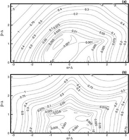
Figure 13.8 shows the local error, £local, contours in the аА – в A plane. In calculating £local, к has been set equal to 1.2. It has been found through numerical experimentation that к = 1.2 is a reasonably good value to use. As readily seen in Figure 13.8, unlike extrapolation, there is no large error even for high wave numbers.

Figure 13.7. A 16-point regular stencil in the form of a square.

Figure 13.8. Contours of local interpolation error, Elocal, in the a A — в A plane for the irregular stencil of Figure 13.6 using the optimized interpolation scheme. (a) at A, (b) at D.

In most aeroacoustics applications, the range of wave numbers that is of interest is -1.0 < a A, в A < 1.0. In order to show error maps with more clarity, only the low wave number portion of the а A – в A plane is shown in the discussions to be followed.

The imposition of order constraints has a significant impact on the local error distribution in the wave number space. Generally speaking, imposing high-order constraints is beneficial in reducing the error in the low wave number region. On the other hand, it tends to cause an increase in error in the high wave number region.

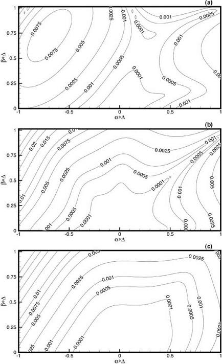
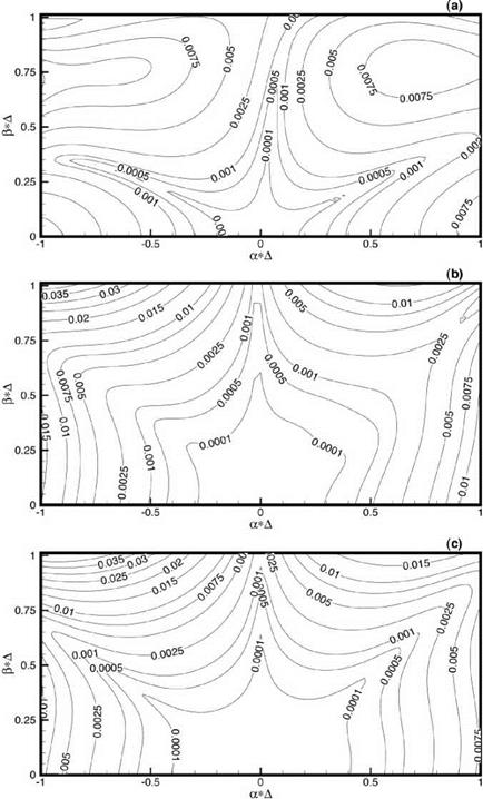
Figures 13.9a-13.9c show the error contour distributions in the а A – в A plane for interpolation to point A using the irregular stencil of Figure 13.6. Figure 13.9a is obtained with the imposition of a second-order constraint. Figures 13.9b and 13.9c are the results with the imposition of a third – and fourth-order constraint, respectively. It is clear from these figures that the best result or least error in the region -0.5 < aA, в A < 0.5 is realized by enforcing the highest-order constraint. On the other hand, if one is interested in keeping the error small over a larger region in wave number space, then the low-order constraint becomes attractive. For point A only the second-order constraint interpolation has an error less than 1 percent over the wave number region of -1.0 < aA, в A < < 1.0. Figures 13.10a-13.10c are for interpolation to point D of the irregular stencil. Again, the error contours of these figures point to the benefit of minimizing interpolation error over the low wave number range by using the maximum order constraints. The error is less than 0.25 percent for |aA |, ^A | < 0.55 (wave length longer than 12.5 mesh points). Again, for the larger wave number range, say -1.0 < aA, в A < 1.0, the second – order constraint has an interpolation error less than 1 percent. Thus, the choice of order constraints depends on the range of wave numbers one wishes to have the error below a specified level. For general usage, the imposition of a medium-order constraint (say second or third order for a 16-point irregular stencil) may be a good compromise.

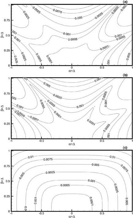
Figure 13.11 shows contours of local interpolation error, £local, at A using the 16- point regular stencil of Figure 13.7. Figures 13.11a-13.11c are subjected to second-, third-, and fourth-order constraints, respectively. Because of regularity of the stencil points, Xj = xk and yj = yk occur repeatedly, there are only four independent values of Xj and yj (j = 1,2,…, 16). This immediately leads to degeneracy in the fourth-order constraints. To show this is, indeed, the case, recall that the interpolation coefficients are to be found by solving Eq. (13.35) BX = d. Here, N is 16. Including the last row of submatrix A, the last 15 rows of matrix B are as follows:

	1		1		1 ••		1	0 …………..	……….. 0
X1	– X0	X2	– X0	X3	– X0 ••	‘ XN	– X0	0 …………..	……….. 0
У1	– У0	y2	– У0	У3	– У0 ••	‘ УN	– У0	0 …………..	……….. 0
(X1 ■	– X0)2	(X2	– X0)2	(X3 ■	– X0)2 "	‘ (XN	1 * О	0 …………..	……….. 0
(У1 ■	– У0 )4	(y2	– У0 )4	(У3 ■	– У0)4 ••	■ CVn	о •• i	0 …………..	……….. 0

If there is no degeneracy, these fifteen row vectors must be linearly independent. But this is not the case as shown below.

Consider the following five of the fifteen row vectors:

	1		1		1		1	0 ■■■ ■	■ ■■■ 0"
x1	– x0	x2	– x 0	x3	– x0 ■	■ xN	– x 0	0 ■■■ ■	■ ■ ■ ■ 0
(X1	– x0 )2	(x2	– x0)2	(x3	– x0)2 ■	■ (xN	– x0)2	0 ■■■ ■	■ ■ ■ ■ 0
(xx	– x0 )3	(x2	– x0)3	(x3	– x0)3 ■	■ (xN	– x0)3	0 ■■■ ■	■ ■ ■ ■ 0
_(xx	– x0 ) 4	(x2	– x 0 ) 4	(x3	– x0)4 ‘	■ (xN	– x 0 ) 4	0 ■■■ ■	■ ■ ■ ■ 0_

Since there are only four independent х-’s, there are only four independent col­umn vectors. It follows that there are only four independent row vectors as well. Similarly, there is also one degeneracy because there are only four independent val­ues of y coordinates. To impose fourth-order constraint on the interpolation scheme, only 13 linearly independent conditions are imposed. Figure 13.11c is computed with only 13 constraints.

On comparing Figures 13.11a-13.11c, it is clear that the case with fourth-order constraints turns out to have slightly more error than those with lower-order con­straints. On the other hand, the cases with second-order and third-order constraints are about the same. Figures 13.12a-13.12c show similar error contours for the point D of Figure 13.7. Again because of degeneracy with the fourth-order constraints only thirteen conditions are used in the optimization procedure. An inspection of these figures suggests that there are only minor differences among them. If minor differences in the distribution of interpolation error is acceptable, then the use of the second-order constraints would suffice when a highly regular stencil is used.