COMBINED OPTIMIZATION AND INVERSE DESIGN. OF 3-D AERODYNAMIC SHAPES

G. S. Dulikravich

The Pennsylvania State University, University Park, PA, USA

12.1 Introduction

The main drawback of using constrained optimization in 3-D aerodynamic shape design is that it requires anywhere from hundreds to tens of thousands of calls to a 3-D flow-field analysis code. Since certain general 3-D aerodynamic shape inverse design methodologies require only a few calls to a modified 3-D flow-field analysis code, it would be highly desirable to create a hybrid new design algorithm that would combine some of the best features of both approaches while requiring less computing time than a few dozen calls to the 3-D flow-field analysis code. We will discuss two such hybrid design formulations that have been proven to work and are dis­tinctly different from each other.

12.2 Target Pressure Optimization Followed by an

Inverse Design

The unique feature of this concept (204). (205) is that it offers the most economical approach to constrained aerodynamic shape optimization. It consists of two steps: surface pressure con­strained optimization follow ed by an inverse shape design. This approach avoids most of the lim­itations of the inverse shape design while requinng considerably less computing time than the direct geometry optimization.

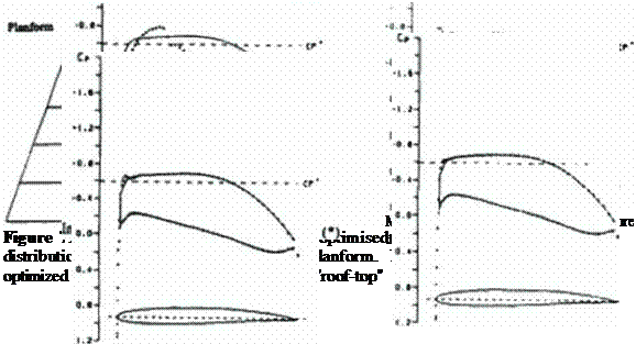
Surface pressure optimization phase of this design approach starts by parameterizing the initial surface pressure distribution using (3-splines (206). Typically, between five and ten control points in the ^-spline representation are sufficient to describe the pressure distribution on the upper surface and the similarly small number of control points is sufficient for represen­tation of the pressure distribution on the lower surface of a two-dimensional (2-D) section of the 3-D object. For example, if 7 control points are used to parameterize the upper surface pressure distribution and 7 control points are used to parameterize the lower surface pressure distribution (Figure 78). then 4 control points will have to be used to fix the locations of leading and trailing edge stagnation points. Constraints can be introduced at this stage by specifying the slopes of the pressure distribution at the leading edge. This will require fixing one additional control point on the upper and the lower surface pressure distribution (204]. The steeper the leading edge pressure distribution variation, the larger the leading edge radius of the resulting 2-D aero­dynamic section will be. The optimization of the constrained surface pressure distribution can then be achieved (207]. (208] by optimizing the 8 "floating” control points each defined by its x – coordinatc and the corresponding value of pressure. The optimization is thus performed on sur­face pressure distribution, not on the actual aerodynamic shape.

This means that the perturbations introduced in the surface pressure distribution during the optimization will have to be somehow related to the global objectives like aerodynamic lift, drag. etc. These global aerodynamic parameters depend on the geometric shape of the object and on the pressure distribution on its surface. It is therefore necessary to relate the geometry of the object and the surface pressure distribution. This is precisely what a typical flow-field anal­ysis code should do except for the fact that geometry of the object is not known yet. A possibil­ity would be to run an inverse shape design code for each surface pressure perturbation and then to integrate the surface pressure in order to evaluate the corresponding lift. drag. etc. This is

obviously an unacceptably, inefficient approach.

Instead, the guessed surface pressure distribution can be optimized without ever calling a flow-field analysis code or the inverse shape design code. To accomplish this, use is made of extremely efficient approximate relations 1209). |2I0| relating the integrated surface pressure distnbution and the object s maximum relative thickness (209), specified location of the flow transition points, and the aerodynamic drag with any of the classical boundary layer solutions (210). Then, the optimization of the few coefficients, for example, of {3-spline parameterization of the surface pressure distnbution curves on each 2 D section can be performed reliably and economically using an optimization algorithm [211], (204). (212). Optimization of the surface pressure distnbution parameters, instead of directly optimizing the 3-D geometry parameters, has several advantages: the total number of optimization variables is reduced, the range of (3- splinc coefficient variations can be large, the design space docs not have an excessive number of local minima, and the sensitivity derivatives do not have discontinuities This procedure easily accepts constraints on surface pressure distribution such as the desired slopes of the curves at the leading and trailing edges, the maximum value of negative coefficient of pressure, a condi­tion that the surface pressure distribution curves on the upper and the lower surface never cross each other thus avoiding locally negative lift force. These optimization tasks can be reliably achieved using a genetic evolution optimization algorithm (204). although an even more reliable and computationally faster approach would be to use a hybrid genetic/gradient search optimiza­tion algorithm (212). (213).

The second phase of this combined 3-D shape design procedure utilizes the optimized surface pressure distribution and any of the fast inverse shape design algorithms (214). (204), (215) to find the corresponding 3-D configuration (Figure 79).

The entire two-step design algorithm requires a minimum development lime since (3- spline discretization codes, constrained optimization codes, flow-field analysis codes, and inverse design codes are available to most aerodynamicists. If the optimized surface pressure distribution results in a 3-D geometry which violates some of the local geometric constraints, the computed pressure at the constrained points can be used instead of the optimized local pres­sure Moreover, this approach gives the designer a partial control of the key elements of the design by asking him to specify a few key bounding features of the "good" surface pressure dis­tribution and then lolling the robust and fast optimizer find (he details of the optimal pressure distribution. Using this approach to shape optimization the designer also has the ability to visu­ally control and terminate or restart the design process if he decides that the values of some of his specified constraints could be improved.

The method offers the most economical and robust approach to 3-D constrained aero­dynamic shape optimization (Figure 80> that consumes approximately 5 – 10 times the comput­ing time needed by a single 3-D flow-field analysis (204). This is much more cost-effective than (ho classical approach of simultaneously optimizing the surface pressure distribution and the corresponding 3-D geometry w hich costs an equivalent of hundreds and even thousands of flow field analy sis runs.

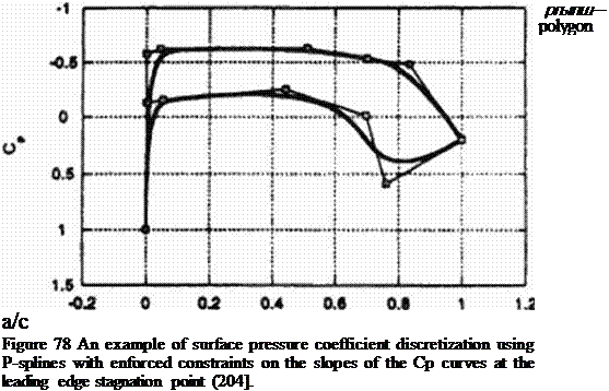
Modified geometry and preuure distribution. F(ntl dittnbution» (*>

(*) after five ucra&oni after not iteration}

Figure 80 An example of a convergence history of target pressure optimization followed by transpiration inverse design [204].