Continuation of a Near-Field Acoustic Solution to the Far Field

By now, it is abundantly clear that all computational aeroacoustics (CAA) simu­lations can only be carried out in a finite, and in most cases, as small as possible, computational domain. A critical problem is how to continue the numerical solution to the far field. In some cases, the acoustic field consists of discrete frequency sound or tones. But in most cases, such as jet noise, the sound field is broadband and ran­dom. In aeroacoustics, most broadband noise is the result of turbulence. Turbulence is random and definitely nondeterministic, and the same is true of the radiated noise. The nondeterministic nature of the noise of turbulence makes its continuation to the far field a much more challenging task.

Mathematically, the problem of extending a near-field acoustic solution to the far field is akin to the mathematical procedure of “analytic continuation” in complex variables. Analytic continuation extends an analytic function defined in a limited domain to a large domain. Because the ideas behind the two problems are similar, the word “continuation” is used here to indicate the objective and intent.

At high Reynolds numbers, a flow is inevitably turbulent. As noted earlier, a turbulent flow is chaotic and random. For a turbulent flow such as that of a high Reynolds number jet, the solution is nonunique. Nonuniqueness is a characteristic of turbulence. Only the statistical averaged quantities are stationary with respect to time. This being the case, it brings forth the question of what physical variables should be continued to the far field. There is also the question of cost in performing the continuation. One may wish to continue the entire turbulence information to the far field, but the computational cost is likely to be prohibitive. Thus, this may not be a good idea. From a practical standpoint, the crucial information one needs in the far field is the noise directivity and spectra. If, indeed, the noise spectra and directivity are the information required in the far field, then a not so expensive computational procedure may be developed to continue this information from the near to the far field. In this chapter only the continuation of the spectra and directivity of turbulence noise are considered.

Turbulent flows are nonlinear, but outside the turbulence region, the velocity and pressure fluctuations are essentially linear. According to the investigation of Phillips (1955) and Stewart (1956), the mean squared fluctuating velocity associated with a turbulent jet or a similar flow decays with an inverse fourth power of the distance from the turbulence region. This prediction has been confirmed by Kibens (1968),

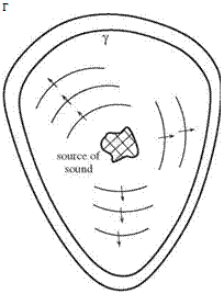
Figure 14.1. Sound generated by a localized source.

Bradbury (1965), and Maestrello (1973) experimentally. Outside the turbulence region, where the linearized Euler equations are valid, the mean squared velocity fluctuations decay with a second power with distance. This is the beginning of the acoustic near field. It will be assumed that the turbulent flow computation extends beyond the turbulence-irrotational boundary to the acoustic near field in the physical domain. The task of interest and the principal objective of this chapter are to develop a robust computational method to continue the numerical solution from the acoustic near field to the far field.