Sliding Interface Problem in Three Dimensions

As an example of the use of overset grids in three dimensions, consider the propagation of a small-amplitude three-dimensional spherically symmetric acoustic pulse across a sliding interface. This problem is chosen because an exact solution
(linearized) is available for comparison. On taking into account spherical symmetry, the linearized dimensionless momentum and energy equations are

9 p 1 d 2

+ (R2v) = 0,

dt R2 dR

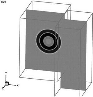
Figure 13.23. Computed pressure con­tours in the x — y plane at t = 30.

where R is the radial coordinate and v is the radial velocity. The initial conditions at t = 0 corresponding to a radially symmetric Gaussian pressure pulse with a half-width b are

(13.47)

(13.48)

The exact solution of Eqs. (13.49), (13.50), and (13.51), which is bounded at R = 0, is

Numerical computation of this problem in three-dimensional Cartesian coor­dinates using the 7-point stencil DRP scheme and the optimized multidimensional interpolation method for data transfer across the sliding interface has been carried out. This may be regarded as a three-dimensional extension of the acoustic pulse problem of Section 13.4.1. The major difference is that there are now 64 points, 4 x 4 x 4, in the interpolation stencil. Again, as in the two-dimensional problem, a

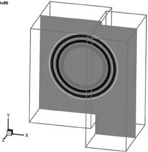
Figure 13.24. Computed pressure con­tours in the x — y plane at t = 60.

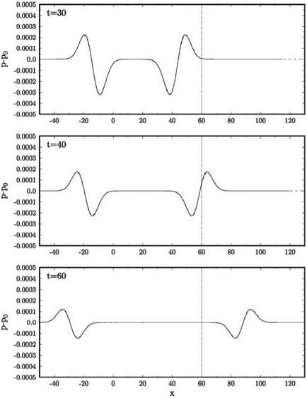
uniform mean flow at Mach 0.5 in the x direction is included (the exact solution is obtained by applying a moving coordinate transformation to solution (13.52)). The sliding grid is taken to be moving in the z direction at a Mach number of 0.4. The full Euler equations are computed. The initial conditions are as given in Eqs. (13.47) and (13.48). The initial pressure pulse has a half-width of six mesh spacings and an intensity with e = 0.005. The pulse is centered at the origin of the coordinate system. The sliding interface is located at x = 60.

Figures 13.23 and 13.24 show the computed pressure contours in the x — y plane at time t = 30 and 60. The acoustic pulse expands spherically at a dimensionless speed

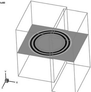Figure 13.25. Computed pressure con­tours in the x — z plane at t = 60.

Figure 13.26. Comparisons of computed waveforms with exact solution at t = 30, 40, and 60.

of unity and is simultaneously convected in the downstream direction by the mean flow at a speed of 0.5. At time t = 30, the pulse has not reached the sliding interface. At t = 60, part of the pulse has crossed the sliding interface into the downstream moving grid. The computed pressure contours remain circular. Figure 13.25 shows the pressure contours at t = 60 in the x – z plane. Again, the contours are circles centered at x = 30, z = 0. Figure 13.26 shows the computed wave form in the x – y plane at t = 30, 40, and 60. Plotted in this figure also are the exact wave forms, but they cannot be detected because they differ from the computed solution by less than the thickness of the lines.

Finally, it is worthwhile to point out that overset grids method may also be used for computing the solutions of moving boundary problems. In such applications, a stationary grid and a moving grid attached to a moving object are used. For this type of problem, the overlapping grids change constantly with time. As a result, a good deal of effort is needed in locating the overlapping grids.

EXERCISES

13.1. To find the values of P in Exercise 11.2, one may use the multidimensional optimized interpolation method. Compare the result of this method and the two – step line interpolation method of Exercise 11.2.

13.2. Use the overset grids method to compute the scattered sound field generated by a plane incident wave train impinging on two cylinders. An exact solution can be found following the method of Sherer (Proceedings of the Fourth CAA Workshop on Benchmark Problems, NASA CP 2004-212954, September 2004).

13.3. (A moving boundary problem) Sound is generated by an oscillating cylinder of diameter D immersed in an inviscid, non-heat-conducting gas. The center of the cylinder lies on the x-axis and is moving so that at time t it is located at x = F(t), where F(t) is a periodic function. One way to compute the radiated sound is to use the overset grids method. This will involve several steps.

Step (1). Use a cylindrical grid fixed to the cylinder as in Figure 13.2. In the cylinder-fixed coordinate system, the governing equations have to be derived by performing a change in coordinates to the Euler and energy equations. Let (xc, yc) be the cylinder-fixed Cartesian coordinates centered at the center of the cylinder. Then,

x = xc + F (t )> y = Ус-

The relationships between (xc, yc) and cylindrical coordinates (rc, Qc) are

xc = rc cos(0cX yc = rc sin(0c)-

Now, transform the Euler and energy equations to the cylinder-fixed coordinates. The value of (u, v, p, p) on the cylindrical mesh are computed by solving this set of equations. Note that u is still the velocity component in the x direction with respect to the background-fixed coordinates. If uc is the component relative to the cylinder, then, uc = u – dF.

Step (2). Use a Cartesian coordinates system to compute the values of (u, v, p, p) in the background coordinates. The background mesh has a square hole similar to that of Figure 13.1. This hole moves with the cylinder in the course of time.

Step (3). The values of (u, v, p, p) on the outer most three rings of the cylindrical mesh are not computed. They are obtained by interpolation from the values of those on the background mesh. Similarly, those values at the innermost three rows and three columns of the square hole are not computed. They are to be found by interpolation from the values on the cylindrical mesh.

Develop a computational strategy for performing the acoustic radiation compu­tation.

Appendix 13A. Computation of the Values of the Elements of Matrix A as Xj ^ xk

As alluded to previously, when the stencil points are aligned on a coordinate line, the limit form of the matrix elements as given by Eqs. (13.16) and (13.20) are to be used; e. g.,

Д sin( )

lim ———————— = к.

Xi^Xk (xj – Xk)

However, for points very nearly aligned, direct numerical evaluation of the matrix or vector elements is not recommended because of the division by a small number. Instead, we advise that the limit values be used whenever |x;- – xk| < e. To find a suitable value of e, let us consider the error incurred when (Д/(х;- – xk))sin(K (x;­- xk)/ Д) is approximated by its limit value к, where |x;- – xk| < e. Let Z = (x;- –

хк)/Д, we have by Taylor series expansion,

It is easy to establish

Thus, the relative error of using the limit value to approximate the relevant parts of a matrix element is less than (к2/3!)(е/Д)2. We recommend to take e/Д = 10-5 for к = 1.2. In this case, the relative error is less than 2.4 x 10-11. This is an extremely small error.

Appendix 13B. Derivation of an Exact Solution for the Scattering of an Acoustic Pulse by a Circular Cylinder

In this appendix, an exact analytical solution for the scattering of an acoustic pulse by a circular cylinder is derived. The solution provided in the Proceedings of the Second CAA Workshop on Benchmark Problems has an error.

Let the cylinder be centered at (x, y) = (0, 0) with a radius r0 and the acoustic pulse be initialized as

p(x, y, 0) = e-b[(x-Xs)2+(y-ys)2], u = v = 0 at t = 0, (13.53)

where p is the pressure, (u, v) is the velocity, and b = (ln2)/d2. Here, d is the half­width of the pulse, and (xs, ys) is the center of the initial pulse. The solution will be found in terms of a velocity potential ф defined as

Let

Ф(Х, y, t) = Фі(x, y, t) + Фг(x, y, t),

where Фі(х, y, t) represents the wave generated by the pulse in the free space and Фг(х, y, t) represents the wave reflected by the cylinder. The solution for Ф(х, y, t) is

TO

j Ai (x, y, ш) e~iotdo 0

where

and rs = у (x – xs)2 + (y – ys)2. Here, Im{} and Re{} denote the imaginary and real part of {}, respectively, and Jk denotes the Bessel function of order k.

To find Фг, on following Eq. (13.55), the solution may be taken to have the following form:

in which Ar(x, y, ш) satisfies the Helmholtz equation

and the following solid wall boundary condition on the cylinder,

Ar can be solved by separation of variables in the polar coordinates (r, в), which gives the following expansion: (ys = 0)

TO

Ar (x, y, oj) = ^2 Ck (ш) Hk ) (roj) cos (кв). (13.59)

k=0

In Eq. (13.59), H(1) is the Hankel function of the first kind of order k. The expansion in Eq. (13.59) ensures that Фг will satisfy the far-field radiation condition. Then, the boundary condition Eq. (13.58) leads to

(13.60)

where

where e0 = 1 and ck = 2 for k = 0.

Finally, the total pressure field can be found as follows:

TO

J (At(x, y, ю) + Ar(x, y, m))me-imtdm 0

where Ai(x, y, ю) is given by Eq. (13.56) and Ar(x, y, ю) is given by Eq. (13.59).