Determination of Steady Thermal Boundary Conditions

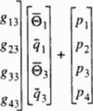
Inverse determination of unknown steady thermal boundary conditions when temperature and heat flux data arc not available on certain boundaries is an ill-posed problem [256)-(264) (Figure 85). In this case, additional overspecified measurement data involving both temperature and heat flux are required on some other, more accessible boundaries or at a finite number of points within the domain. For example, when using a BF. M algorithm, if at all four vertices designated with subscripts 1,2,3. and 4 of a quadrilateral computational gnd cell the heat sources pi are known.

at two vertices both temperature 0 as 0 and heat flux q = q arc known, while at the re-

maining two vertices neither Q or q is known, the boundary integral equation becomes

(88)

Here, coefficients of (h) and |g) matrices arc all known because they depend on gcomet nc relations and the configuration is known. In order to solve this set. all of the unknowns will be collected on the right-hand side, while all of the knowns are assembled on the left. A simple algebraic manipulation yields the following set:

— m

*11 ~#,2 *13 ”#i4

*21 ”#22 *23 ”#24 » •

*31 “#32 *33 ”#34 *41 “#42 *43 -#44

Since (he entire right-hand side is known, it may he reformulated as a vector of known*. {¥). The left-hand side remains in the form [A){X}. Also, additional equations may be added to the equation set if. for example, temperature or heat flux measurements are known at certain locations within the domain. In general, the geometric coefficient matrix [Л] will be non-square and highly ill-conditioned. Most matrix solvers will not work well enough to pro­duce a correct solution. There exists a very powerful technique for dealing with sets of equa­tions that are either singular or very close to singular These techniques, known as Singular Value Decomposition (SVD) methods |265], arc widely used in solving most linear least squares problems. Thus, using an SVD algorithm it is possible to solve for the unknown surface temperatures and heat fluxes very accurately and non-iteratiscly. If the general formulation of the problem is to be done with finite elements or any other numerical technique instead of BEM, the inverse boundary condition determination problem would become iterative and would require special regularization methods to keep it stable.