GLOBAL NONLINEAR ANALYTICAL MODELING

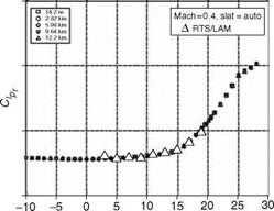
a (°) FIGURE 9.6 A compound derivative from RTS data using partitioning method on LAM data for FA2.

characteristics for large AOA range. Also, at certain flight conditions, it may not be possible to trim the aircraft and obtain the point models from the flight test data. Thus, global models obtained from the wind tunnel and flight data can constitute a total aerodynamic database, which would be a good source for validation of flight control performance, flight envelope expansion, and wind-tunnel aero database [31,32]. This aero database can be updated if required based on the results from flight test data analysis. A global model with a gradient and a large range of validity can replace many local models in the flight envelope. In addition, the partial derivatives of the global analytical model would provide point models (at trim conditions) that can be used in control system design. Multivariate orthogonal functions are very useful for global modeling of aerodynamic coefficients [31]. A minimum predicted squared error (PSE) criterion [1] can be used to determine the orthogonal functions to be included in the global model. The other criteria used are the sum of the conventional mean squared error (MSE) and an over-fit penalty (OFP) [33]. Each orthogonal function included in the global model can be decomposed into an ordinary polyno­mial in independent variables. Thus, the global model can assume the form of a truncated power series expansion, providing an insight into the physical relationship between the aerodynamic coefficients and independent variables. The orthogonal functions approach also allows for an easy upgrading of the model with the newly acquired flight data. Alternatively, the spline functions can be used to fit the flight – determined derivatives, padded with linear model derivative values obtained from wind-tunnel data, to determine global models of force and moment coefficients as functions of trim AOA and Mach number [34]. A spline is a smooth piecewise polynomial of degree m, with the function values and derivatives agreeing at the points where the piecewise polynomials join. These points are called ‘‘knots,’’ defined by the value of their projection on to the plane or axis of independent variables.

For the polynomial splines of degree m, a single variable function f(a) can be approximated in the interval a 2 [a0, amax] as

(9.70)

with

(a – a,)™ = (a – a,)m if (a > a,)

= 0 if (a < a,)

ab a2,ak are knots obeying the condition a0 < a1 < a2 < • •• < ak < amax and the coefficients Ch and D, are constants. A function of two variables f (a, b) can be approximated in the range, a Є [a0, amax] and b Є [bo, bmax], using polynomial splines in two variables. First-order splines are generally adequate for modeling the nondimensional derivatives of an aircraft. It is assumed that the spline polynomial of an aerodynamic derivative C, which is a function of a and Mach number, can be expressed as shown below:

k I

C(a, M) = Я00 + «0ia + ящМ + a\aM + E bi(a – a,)1 + Ec<M – M)1

i=1 j=1

k l

+ X) Edj(a – ai)1(M – Mj)1 (9.71)

i=1 j=1

Here, the constants a00, …a11, b,, c,-, and dj are to be determined. A higher order may be used if the degree of nonlinearity in the data is believed to be high. The LS regression matrix, computed using the values of the nondimensional derivative and the independent variables a and M, is orthogonalized using the Gram-Schimdt procedure. The minimum PSE metric is used to determine the model structure and the global model parameters are estimated using the LS regression method.

The global models of the nondimensional derivatives of a high-performance aircraft were identified using the splines technique and validated over an AOA range of 0°-22° and Mach range of 0.2-0.9 [33]. The GM of Cma from splines comprises 25 terms with the knots placed at every 1° a from 0° to 22°, and the Mach knots were placed at intervals of 0.1 between 0.2 and 0.9 Mach. According to Equation 9.70, as a increases, each spline function (a – ai) contributes less than the previous function, allowing for different values of derivatives to be computed for different values of a. The static validation of GMs is done by comparing them with several point values. The results of model fitting with splines are shown in Figures 9.7 through 9.9. GMs were validated dynamically using data from the 6DOF nonlinear simulation.