Surface Green’s Function: Normal Velocity as the Matching Variable

Instead of using surface pressure as the variable for continuation to the far field, an equally good variable to use is the velocity component normal to the surface or the normal pressure gradient. If this choice is made, the appropriate surface Green’s function is given by solution of the following problem (a superscript “G” will be used to denote this Green’s function):

д V(G) Po dt +VP(G) =o	(14.25)
djP^- + YPoV • v(G) = o,	(14.26)

On surface Г, i. e., g = go, the boundary condition is

v(G)(x, t; to, no, So, to) = s(t — toЖп — По)Ж — to)•

To find v^ (x, t; to, no, go, t), it is advantageous to introduce a velocity potential Ф(^ defined by

v(G) = v ф(^, p(G) = — po——- . (14.28)

dt

Eq. (14.28) satisfies Eq. (14.25) identically. Substitution of Eq. (14.28) into Eq. (14.26), the governing equation for Ф(^ is found to be

1 d 2ф^)

2 v2 Ф(^ = o. (14.29)

ao dt2

The surface boundary condition on g = go is found by inserting expression (14.28) into Eq. (14.27). This yields

дФ^)

-— = S(i — to )S(n — no )S(t — to), (14.3o)

where n is the unit outward pointing normal of surface Г.

Suppose Ф(С)(х, t; ^0,v0,g0, t0) is found. Let vn (f0, n0, t0) be the prescribed

normal velocity on Г, then the velocity potential (v = V Ф and p = — —дф) is

p0 dt

given by

TO TO TO

/// Ф )(x, t; %0’ n0’ ?0’ t0)vn (^0’ n0’ t0) d^0 dn0 dt0- (14.31)

-TO – TO – TO

The pressure field may be computed by differentiating Eq. (14.31) with respect to t, i. e.,

By means of Eq. (14.28), this expression may be rewritten as

To illustrate the construction and use of surface Green’s function p(G), con­sider again the case of Г in the form of an infinite circular cylindrical surface as shown in Figure (14.2). The governing equation for Ф(^ is Eq. (14.29). In cylindrical coordinates, the equation and boundary condition for Ф(^ are

At r = ^

ЭФ(С) = 3(ф – ф0)8(x — xQ)8(t -10) 9 r D/2

Just as in Section 14.2, the solution of this problem may be constructed by first applying Fourier transforms to x and t and then expanding the solution as a Fourier series in (ф — ф0). On denoting the Fourier transform by a ~ over the variable and the amplitude function of the mth term in the Fourier series by a subscript m, the solution takes on the following form:

TO

Ф(G) = Фтеіт(ф—ф0). (14.36)

— TO

It is straightforward to find that

where H<m) and Hm are the mth order Hankel function and its derivative. The
inverting the Fourier transforms, it is readily found that

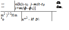
Ф(G)(r,<p, x; фо, Xq, to)

For radiation to the far field, the k integral in Eq. (14.37) may be evaluated asymptotically (method of stationary phase) by first switching to spherical polar coordinates as in Section 14.2. In so doing, and upon using Eq. (14.28), it is found that

p (а)(Я, в,Ф, t; Фо, Xq, to)

R^to

To demonstrate that Eq. (14.38) is the correct surface Green’s function with vn as the matching variable, the time periodic monopole source problem of Sec­tion 14.2 is again considered. For a monopole source located at the origin with angular frequency Q, the pressure field is given by Eq. (14.19). By means of the radial (R direction) momentum equation, it is easy to find that the radial velocity vR associated with the acoustic field is

The component of vR in the direction normal to the cylindrical surface and on the cylindrical surface, r = D/2 is

where R0 = (D + x2 )1/2 and sin в = D. x0 and t0 are the source coordinate and time.

Now, on inserting p(G) from Eq. (14.38) and vn from Eq. (14.40) into Eq. (14.33), the radiated pressure field at R ^ to is given by

p (R, в, ф, t)) =

R^to

The integrals over dt0 and dф0 can easily be evaluated to yield

ю 2n

I e*(“-Q)to dt0 = 2nS (a – Q), J eim(^—фо^ф0 = 2П ^.

-ю 0

Thus, upon integration over dt0, d(p0, and da and on summing over m, Eq. (14.41) becomes

The remaining integral of Eq. (14.42) can be evaluated in closed form by differ­entiating formula (14.23) with respect to parameter a. By means of this formula, it is easy to find that the pressure field becomes

iQ R-t

This is just the acoustic field of a time periodic monopole.