FUZZY LOGIC-BASED METHODS FOR ESTIMATION

In recent times, approaches for parameter and state estimation using ANNs and fuzzy logic have improved. Here, some approaches are briefly discussed and a few results are given.

9.9.1 ANFIS for Parameter Estimation

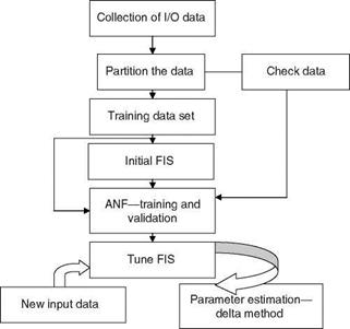
An ANFIS (the adaptive neuro-fuzzy inference system of MATLAB; MATLAB is a registered trademark of MathWorks, Inc.) for parameter estimation uses the rule – based procedure to represent the system behavior in the absence of a precise model of the system and uses the I/O data to determine the membership function’s parameters (constants). It consists of the fuzzy inference system (FIS) whose membership function’s parameters are tuned using either a back propagation algorithm or in combination with the LS method. These parameters will change through the learning process. The computation of these parameters is facilitated by a gradient vector, which provides a measure of how well the FIS models the I/O data for a given set of parameters. Once the gradient vector is obtained, any optimization routine can be applied to adjust the parameters to reduce the error measure defined by the sum of the squared difference of the actual and desired outputs. The membership function is adaptively tuned/determined using ANN and the I/O data of the given system. The FIS is shown in Figure 2.19. The process of system parameter estimation using ANFIS is depicted in Figure 9.11. The steps

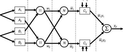
involved in the process are depicted in Figure 9.12. Consider a fuzzy system with the rule base: (1) If щ is Aj and u2 is Bb then yj = c11u1 + c12u2 + c10; if mj is A2 and u2 is B2, then y2 = c21uj + c22u2 + c20. Here, ub u2 are crisp/non-fuzzy inputs, and y is the desired output. Let the membership functions of fuzzy sets Ai, Bi, i = 1,2 be mA, mB. ‘ pi’’ is the product operator to combine the AND process of sets A and B, and N is the normalization. Cs are the output membership function parameters. The steps are given as (1) each neuron ‘‘i’’ in layer 1 is adaptive with a parametric activation function. Its output is the grade of membership function to which the given input satisfies the membership function, i. e., mA, mB. A generalized member­ship function m(u) = 1+|U-cj2b is used and the parameters (a, b, c) are premise

parameters; (2) every node in layer 2 is a fixed node, whose output (wi) is the product П of all incoming signals: w1 = mA (u1)mB (u2), i = 1,2; (3) output of layer 3 for each node is the ratio of the ith rule’s firing strength relative to the sum of all rules’ firing strengths: w, = www ; (4) every node in layer4 is an adaptive node with a node output: Wj-yj = w!(c! lu1 + ci2u2 + ci0), i = 1, 2. Here, c is the consequent parameters; and finally (5) every node in layer 5 is a fixed node, which sums all incoming signals yp = w1y1 + w2y2, where yp is the predicted output. When the parameters of the premise are fixed, the overall output is a linear combination of the consequent parameters. The output (linear in the consequent parameters) can be written as

yp = w 1y1 + W 2 y2 = w 1(c11U1 + c12U2 + c10) + W2(c21U1 + c22U2 + c2o)
= (w 1U1)c11 + (w1U2)c12 + w 1c10 + (w 2 U1)c21 + (w 2U2 )c22 + w 2c20

by the LS method. In a backward pass, the error signals propagate backward and the premise parameters are updated by a gradient descent method. The steps involved are (1) Generation of initial FIS by using INITFIS = genfis1(TRNDATA). ‘‘TRNDATA’’ is a matrix with N + 1 columns, where the first N columns contain data for each FIS, and the last column contains the output data. INITFIS is a single output FIS. (2) Training of FIS: [FIS, ERROR, STEPSIZE, CHKFIS, CHKERROR] = anfis(TRNDATA, INITFIS, TRNOPT, DISPOPT, CHKDATA). Here, vector TRNOPT represents training options, vector DISPOPT represents display options during training, CHKDATA prevents overfitting of the training data set, and CHKFIS is the final tuned FIS.

Example 9.2

Generate simulated data using the equation y = a + bxi + cx2, with a = 1, b = 2, and c = 1. Estimate the parameters a, b, c using ANFIS and the delta method.

Solution

The simulated data are generated and partitioned as training and check data sets. Then the training data are used to obtain tuned FIS, which is validated with the help of the check data set. The tuned FIS is, in turn, used to predict the system output for new input data of the same class and parameters estimated using the delta method. The MATLAB routines are given in ‘‘ExampSolSW/Example 9.2ANFISPEstm.’’ The results are shown in Table 9.14.