The Adjoint Green’s Function

Oftentimes, the surface geometry one encounters does not fit a separable coordinate system. For these cases, the surface Green’s function usually cannot be found easily. For such a surface geometry, one may use the adjoint Green’s function and the reciprocity relation.

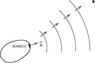
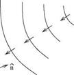
In many branches of mechanics, the reciprocity principle applies. However, the existence of a reciprocity principle has not been fully exploited in the fields of acoustics and fluid dynamics. Some earlier works that utilized reciprocity are Cho (1980), Howe (1975,1981), Dowling (1983), and Tam and Auriault (1998) in acous­tics; Roberts (1960), Eckhaus (1965), and Chardrasekhar (1989) in hydrodynamic stability; and Hill (1995) in receptivity problems. To fix ideas on reciprocity, con­sider a time periodic point source of sound located at xs as shown in Figure 14.5(a). Let G(x0, xs, a) be the pressure associated with the sound field measured by an observer at x0. The time factor e-iat has been omitted. Mathematically, G(x0, xs, a) is the Green’s function of the Helmholtz equation and a is the angular frequency of oscillations. (Note: the notation that the first argument of the Green’s function is the location of the observer and the second argument is the location of the source is retained here.) Now, if the location of the sound source and that of the observer is interchanged as shown in Figure 14.5(b). Clearly, by symmetry, the pressure mea­sured by the observer now at xs while the source is at x0 is the same as before. That is,

G(x0, xs, a) = G(xs, x0, a). (14.43)

Eq. (14.43) is simply a statement that the Green’s function G(x0, xs, a) is self­adjoint. It is the reciprocity relation.

Figure 14.5. An acoustic source and an observer form a self-adjoint system.

X

Observer at x

s

For a surface source and a far-field observer as shown in Figure 14.6(a) a reci­procity relation exists. The problem is, however, not self-adjoint. The adjoint Green’s function is not governed by Eqs. (14.8) and (14.9). The boundary condition is not Eq. (14.10). These equations, referred to as the adjoint equations, may easily be derived in the frequency domain.

There is a significant advantage in using adjoint Green’s function instead of the direct Green’s function when an analytical formula for the Green’s function cannot be found. Suppose the far-field sound in the direction of в produced by surface sources as shown in Figure 14.7a is to be found. To determine the total far-field radiation, the radiation from each surface sources such as A, B, and C in Figure 14.7 has to be calculated and then summed. That is, the surface Green’s functions at A, B, and C and other surface points have to be separately computed. In the absence of an analytical formula, this would be a tedious and laborious effort. On the other hand, if

to source

Figure 14.7. (a) Direct surface Green’s function has to be found for every surface point on surface Г for radiation in the direction в. (b) The adjoint Green’s function for all surface points is the solution of a single scattering problem with the incident wave coming from a distant source in direction в.

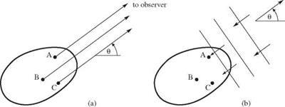
the adjoint formulation is used the situation is different. Since the source point is now in the far field, the sound waves from the far-field source near surface Г are plane waves. The adjoint Green’s function is, therefore, the solution of a simple scattering problem by surface Г. The scattering problem needs to be computed only once. By the reciprocity relation, the values of the direct Green’s function for radiation from every point on surface Г to the far-field point is found simultaneously in one single calculation of the scattered wave solution.

The Fourier transform of Eqs. (14.8), (14.9), and boundary condition (14.10) in time t are

— iop0V(g) + V p(g) = 0 (14.44)

– iop(g) + yP0V ■ v(g) = 0, (14.45)

On Г or 5 = 50,

p(g(x, op $0, П0, 50, t) = 2ns($ — $0Жп — П0Ушг (14.46)

To find the adjoint system of equations to Eq. (14.44) and (14.45), multiply Eq. (14.44) by v(a)■ and Eq. (14.45) by p(a) (the superscript “a” denotes the adjoint) and integrate over all space outside Г. This yields, after rearranging the terms,

[—iop0v(a) ■ v(g) + V ■ (p(g)v(a)) — p(g)V ■ v(a) — iop(g)p(a))

+ Yp0V ■ (p(a)v/(g) — yp0v(g) ■ Vp(a)]dxdydz = 0. (14.47)

The two divergence terms in Eq. (14.47) may be integrated by means of the Divergence Theorem to become surface integrals over Г. This leads to

flfi —iop0v(a) — yp0Vp(a)] ■ v(g)dxdydz

outside Г

+ i-i°p’«

outside Г

V ■ v(a)]p(g)dxdydz

— U [p(g)v(a) + Yp0p(a)v(g)] ■ n dS = 0.

surface Г

where n is the unit outward pointing normal of surface Г.

Now, the adjoint system is chosen to satisfy the following equations and bound­ary conditions:

– irp0v(a) – Yp0 Vp(a) = 0	(14.49)
irp(a) – V ■ v(a) = 2nS(x – x1 )eirT	(14.50)
On Г or g = g0, p(a) = 0.	(14.51)

By means of this choice of the adjoint system, the integrals of Eq. (14.48) may be easily evaluated. This gives the reciprocity relation as follows:

p(g)(x1;f0, П0> т) = т) (M.52)

where vf’1 = v(a) ■ ii is the component of the adjoint velocity in the direction of outward pointing unit normal ii. Thus, once the adjoint problem is solved, the direct surface Green’s function on the entire surface is found.