Time Periodic Sources

For time periodic sources with time dependence e—iQt, the source function on the conical surface may be written in the following general form:

в = 5, psource(R, Ф0, t0) = *(R>. Ф0)e—iQt0. (14.82)

By Eq. (14.61), the far-field pressure field (R ^ ж) associated with the source is given by

p(g)(R, в, ф; R0, ф0; m, t0)^(R0, ф0)e~imt—iQt°R0 sin 5dm dt0dR0 dф0.

(14.83)

On using p(g) in a Fourier expansion in (ф — ф0), i. e., Eq. (14.75), Eq. (14.83) becomes after integrating over dt0 (giving rise to 2п5(ш — О)) and then upon inte­grating over dm,

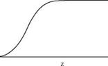Figure 14.11. A typical profile of damping function a(z).

Y

2npm(R, в; R0, n^(R0, ф0)еіт(ф-ф°)-tatR0sinSdR0 йф0,

0 0

(14.84)

where pm (R, в; R0, a) is given by Eq. (14.76). In this form, only two integrations need be evaluated.

As a concrete example, consider a time periodic monopole source located at a distance xc from the apex of a conical surface as shown in Figure 14.12. Let Y be the distance of a point from the monopole source. For a point on the conical surface with a spherical polar coordinates (R0, 5, ф0), Y for this point is given by

Y0 = R0 + x2 – 2R0xc cos 5)2. (14.85)

The pressure field on the conical surface associated with the monopole acoustic source is

Thus, in the notation of Eq. (14.82), the Ф function is

e‘QY0/a0

4nY0

Substitution into Eq. (14.84), the far pressure field of the monopole source, according to the continuation method, is as follows:

In deriving Eq. (14.88), the integral over ф0 has been performed. This integral is zero except for m = 0. Note that p0 is given by Eq. (14.76). The remaining integral

Figure 14.13. Computational domain for the monopole acoustic source.

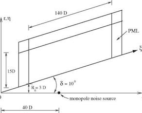
over R0 has to be evaluated numerically. The first step is to compute the adjoint Green’s function v0a) and іл^ in the f – n plane as discussed before. These two quantities are required to compute p0. For the present example, a computational domain with a size as shown in Figure 14.13 is used. The half-apex angle 5 is 10°. Note that a conical surface has no intrinsic length scale. Here, D in Figure 14.13 is taken as the length scale. In the far field, R ^ ж, the directivity factor is defined by

where p is given by Eq. (14.88). For ^ = 1.0, the computed results are shown in

ao

Figures 14.14 and 14.15 for a source located at xc/D = 40.0. The exact solution

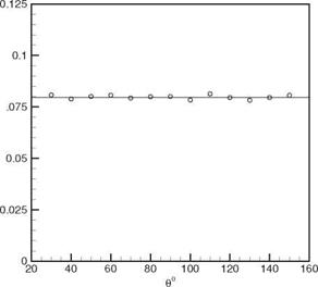Figure 14.14. The computed directivity of a periodic monopole. The straight line is the exact solution.

Figure 14.15. The computed phase of an off-center periodic monopole. Full line is the exact solution.

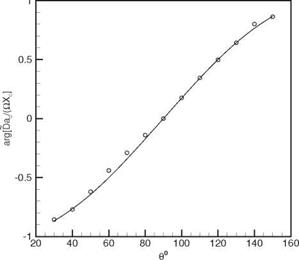_ a D(в, Or)

is D(e ) = |D (в, )| = 4L and arg[ ] = – cos в. The phase factor arises

because the source is not located at the origin of the spherical polar coordinate system. As can be seen, the agreements between the magnitude and phase of the computed results and the exact solution are good. This provides confidence in the numerical method.