Continuation of Broadband Near Acoustic Field on a Conical Surface to the Far Field

An important CAA problem is to compute the noise of a high-speed turbulent jet. Since a computational domain is finite, it extends only to the near acoustic field. To determine the far-field sound, the continuation method developed in the Section

14.6 may now be used. The noise of a turbulent jet is broadband and random. It contains an enormous amount of information. However, for practical purposes, the

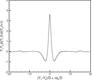
Figure 14.19. The two-point space-time correlation function computed accord­ing to Eq. (14.92).

quantities of interest in the far field are the noise spectra and directivity. For this reason, only the continuation of the noise spectra from the near field to the far field at different angular direction is considered.

In Section 14.5, it was suggested that a good choice of a matching surface Г is a conical surface as shown in Figure 14.8. A method to compute the surface Green’s function p(g) (R, в, ф, t; R0, ф0, t0) through the use of the adjoint Green’s function has also been developed. Let ps(R0, ф0, t0) be the pressure of a turbulent jet measured on the conical surface. The conical surface has a half-apex angle of 5. The far-field pressure is then given by

p(R, в, ф, t)

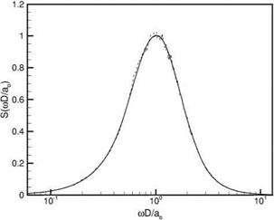Figure 14.20. Comparison between the original (full line) and the computed spectrum (dotted line). The computed spectrum is the Fourier transform of the correlation function F (-f ) given in Figure 14.19.

By Eq. (14.75), the Fourier transform of the surface Green’s function may be expanded in a Fourier series in (ф — ф0), that is,

Now, the far-field noise spectrum, S(R, в, ф, ю), is the Fourier transform of the autocorrelation function, i. e.,

In Eq. (14.95), the angular brackets, {), are the ensemble average of the random variables inside the brackets. Since the sound field is stationary random, the ensemble average and the time average are equal. By means of Eqs. (14.93) to (14.95), the following relation between the spectrum function and the source function can easily be established.

TO TO

E E {ps (R’,ф, t’)ps (r"a" , t"))

m=—to п=—то

x pm (R, в; R’, ю’)pn (R, в; R", ю" )

~—ію'(ї —V )—ію/'(ї—Ґ’)+іт(ф—ф/)+іп(ф—ф/’)—ію/’т+іют x e

x R R’ sin2 SdrdoJdoJ ‘ dt’ dt” dR dR’ dф’ dф”. (14.96)

For jet noise, the surface pressure ps is a stochastic variable that is stationary random in time and homogeneous in the azimuthal variable ф. These properties allow the two-point space-time correlation function to be written as

{ps(R, ф’, t’)ps(R, ф”, t")) = <b(R, R", ф’ — ф”, t’ — t"). (14.97)

On inserting Eq. (14.97) into Eq. (14.96), the far-field spectrum function becomes

2?//f"f £ £ фr —ф"’•’—

J J J J m=—to n=—to

x pm (R, в; R’,ю’)pn (R, в; R ‘,ю")

X е~ію’ (t— ) —ію” (t—t’ )+m (ф—ф1) +іп (ф—ф")—ію"т +іют

X R’R" sin2 Sdr dm dm’ dt’dt" dR’dR" dф’d^’. (14.98)

In the following, it will be shown that, regardless of what the two-point space­time correlation function Ф (R, R", ф’ — ф”, t’ — t”) is, five of the integral and one summation in Eq. (14.98) can be evaluated.

The dr integral may be evaluated in a straightforward manner as follows:

TO

The dt’ and dt" integrals may be evaluated by a change of variables to X = t’ -1", f = t". This gives

TO TO

j j Ф(ІЇ, R" , ф’ – Ф", t’ -1”)e-iot-io’fdt’ dt"

TOTO

= j j Ф(R/, R”,ф’ – ^’,X)e-io X-i(o +o")f df dX

-TO – TO

TO

= 2n5(o’ + o”) j Ф(R/, R",ф’ – ф” ,X)e-io X dX. (14.100)

The d^ and dф" integrals may also be evaluated by a change of variables to

© = ф’ – ф” and Ф = ф”, thus,

2n 2n

j j Ф(ІЇ, R", ©,Х)е-ітф-іпф’d^dф”

00

2n 2n

= j j Ф(R/, R",©,X)e-im©+i(m+n)’l‘dVd©

00

2n

= 2n5m,-n / Ф(ІЇ, R", ©, X)e-im©d©. (14.101)

0

Substitution of Eqs. (14.99) to (14.101) into Eq. (14.98), and upon integrating over do’ and do” and summing over m, the mathematical formula for the noise spectrum is

S(R, в, ф, о)

to to 2n to to

= 4n2ffff ^2 Ф(^, R, ©, X)P-n(R, e; R, – o)pn(R, e; R",o)

0 0 0 – TO n=-TO

x eioX+in©R’R" sin2 5 dXd©dR’dR". (14.102)

Eq. (14.102) is the principal result of this section. Physically, it signifies that the two-point space-time correlation function is the equivalent noise source on the conical surface. If this function is known, either by experimental measurement or by numerical simulation, then the far-field noise spectrum can be computed. Note: the dX and d© integration apply only to the equivalent noise source function. These two operations effectively decompose the source into frequency and azimuthal components.

Eq. (14.102) has been used in the experimental work of Tam, Viswanathan and Pastouchenko (2010) (see also Tam, Pastouchenko and Viswanathan (2010)). They measured the near-field two-point space-time pressure correlation function Ф(№, R", ©, X) of a Mach 1.66 hot jet on a conical surface of 100 half-angle. They
used Eq. (14.102) to determine the far-field noise spectra. They showed that the noise spectra continued from the near-field were in good agreement with the measured far-field spectra.