Linearization of the Potential Equation

The general equation for compressible flows, namely Equation (9.40), can be simplified for flow past slender or planar bodies. Aerofoil, slender bodies of revolution and so on are typical examples for slender bodies. Bodies like wing, where one dimension is smaller than others, are called planar bodies. These bodies introduce small disturbances. The aerofoil contour becomes the stagnation streamline.

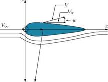
For the aerofoil shown in Figure 9.4, with the exception of nose region, the perturbation velocity w is small everywhere.

9.8.1 Small Perturbation Theory

Assume that the velocity at any point in the flow field is given by the vector sum of the freestream velocity VOT along the x-axis, and the perturbation velocity components u, v and w along x, у and z-directions, respectively. Consider the flow around an aerofoil shown in Figure 9.4. The velocity components around the aerofoil are:

Vx = Vx, + u, Vy = v, Vz = w, (9.42)

where Vx, Vy, Vz are the main flow velocity components and u, v, w are the perturbation (disturbance) velocity components along x, у and z directions, respectively.

Vz w Figure 9.4 Aerofoil in an uniform flow.

The small perturbation theory postulates that the perturbation velocities are small compared to the main velocity components, that is:

u < Уж, v < Уж, w < У

Therefore:

Ух« Уж, у, << Уж, V << Уж. (9.43*)

Now, consider a flow at small angle of attack or yaw as shown in Figure 9.5. Here:

Ух = Уж cos a + u, Уу = Уж sin a + v.

Since the angle of attack a is small, the above equations reduce to:

Ух = Уж + u, Уу = v.

Thus, Equation (9.42) can be used for this case also.

With Equation (9.42), linearization of Equation (9.40) gives:

(1 – И2)фхх + фуу + Фїї = 0, (9.44)

neglecting all higher order terms, where M is the local Mach number. Therefore, Equation (9.41) should be used in solving Equation (9.44).

a

The perturbation velocities may also be written in potential form, as follows: Let ф = фж + q>, where:

фж — : фхх —фжх$ + Фхх. . .

Therefore, ф may be called the disturbance (perturbation) potential and hence the perturbation velocity components are given by:

дф дф дф

u = —, v = —, w = —. дх dy dz

With the assumptions of small perturbation theory, Equation (9.41) can be expressed as:

(

a 2 , , u

— ) = – (y – ) Mж — аж ‘ V ж

(аж )2 — (■ – Y – «-і u )-‘.

Using Binomial theorem, (аж/а)2 can be expressed as:

( ^)! = 1 + (Y – 1) U M + °(m» I )

Substituting the above expression for (аж/а) in the equation:

M = (1 + u) (т) M~,

the relation between the local Mach number M and freestream Mach number Мж may be expressed as (neglecting small terms):

The combination of Equations (9.48) and (9.44) gives:

Equation (9.49) is a nonlinear equation and is valid for subsonic, transonic and supersonic flow under the framework of small perturbations with u ^ Уж, v ^ Уж and w ^ Уж. It is, however, not valid for hypersonic flow even for slender bodies (since u & Уж in the hypersonic flow regime). The equation is called the linearized potential Bow equation, though it is not linear.

Equation (9.49) may also be written as:

Further linearization is possible if:

With this condition Equation (9.50) results in:

This is the fundamental equation governing most of the compressible flow regime. Equation (9.52) is valid only when Equation (9.51) is valid and Equation (9.51) is valid only when the freestream Mach number Ml is sufficiently different from 1. Hence, Equation (9.51) is valid for subsonic and supersonic flows only. For transonic flows, Equation (9.49) can be used. For Ml & 1, Equation (9.49) reduces to:

The nonlinearity of Equation (9.53) makes transonic flow problems much more difficult than subsonic or supersonic flow problems.

Equation (9.52) is elliptic (that is, all terms are positive) for Ml < 1 and hyperbolic (that is, not all terms are positive) for Ml > 1. But in both the cases, the governing differential equation is linear. This is the advantage of Equation (9.52).