Shadowgraph

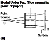
If the flow field is traversed by a light beam (Figure 6.16a), the image that is formed spontaneously on a screen perpendicular to the axis of propagation is called a shadowgraph. If the beam is made parallel by a lens (Figure 6.16b), the shadow will have the same aspect ratio as the model. The images produced are carriers of information so implicit that it is very difficult, if not impossible, to infer density variations from an examination of the image.

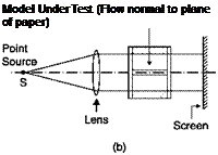The shadowgraph method: (a) divergent light rays; (b) parallel rays

To understand the operating principle of the shadowgraph in detail, the behavior of the index of refraction within the field must be considered. Let AB and CD (Figure 6.17) be the undisturbed paths of two adjacent rays. If there is a variation in the index of refraction, the rays are deflected: if the gradient of the index of refraction, Эл/dx, is constant, i. e. Э2 л/ dx2 = 0, the two rays are deflected by the same angle and remain parallel (Figure 6.17a): the illumination on a screen placed down­stream of the test chamber is uniform. If d2nf dx2 > 0, the deflected rays diverge (Figure 6.17b), because the ray passing in A meets zones with a stronger gradient of index of refraction with respect to the gradient met by the ray passing in C; a darker zone is generated on the screen. Finally, if d2n/dx2 < 0, the rays converge (Figure 6.17c) and a brighter zone is obtained on the screen.

The shadowgraph is successfully used for the visualization of surfaces of discontinuity in the index of refraction (density) like the shock wave, or of layers with strong and variable density gradients (dynamic and thermal boundary layers).

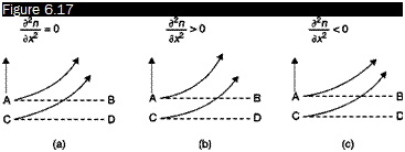Effects of the gradient of refractive index on the deflection of light rays

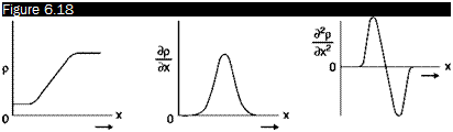Evolution of density, its gradient and the gradient of gradient within a shock wave

Consider, for example, the case of a jump in density across a shock wave (Figure 6.18). In the same figure are shown the evolution of density and of the gradient of the gradient of density inside the wave, con­sidered of finite thickness. In the front of the wave Э2л/dx2 > 0and the screen displays a dark line, in the back д2п/dx2 < 0and the screen displays a bright line. Therefore a shock wave appears on the screen as a succession of two light bands: the first dark and the second bright (Figure 6.19).

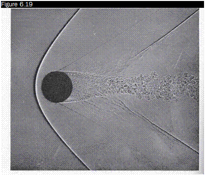Shadowgraph of shock waves and wake on a sphere in a stream at M = 1.6

It can be shown that the contrast of light, C, produced at each point of the screen is given approximately by:

where I is the light intensity and £ is the distance of the disturbance from the screen.

Calculation of density from Equation (6.8) requires a double integration of the local contrast (appropriate devices are needed to measure the light intensity). Moreover, Equation (6.8) becomes less reliable in the description of phenomena that are best viewed with the shadowgraph (i. e. discontinuities in the value of the index of refraction). In fact, large variations in the density gradient will produce, starting from a certain distance from the phenomenon, an intersection of the various rays that destroy the correspondence between points of the test field and the image obtained on the screen that is the basis of Equation (6.8).

The shadowgraph is very simple from the viewpoint of the optical components required, and is useful for the visualization of fluids in which there are discontinuities in density, but it is essentially a qualitative method as the calculation of the distribution of the index of refraction from Equation (6.8) seems rather difficult, if not impossible. One can say briefly that with this method small changes in n are not detected and large variations in n cannot be calculated.