Two-Dimensional Flow: Prandtl-Glauert Rule for Subsonic Flow

9.13.1 The Prandtl-Glauert Transformations

Prandtl and Glauert have shown that it is possible to relate the solution of compressible flow about a body to incompressible flow solution.

The transformation from one to another is achieved in the following manner: Laplace equation for two-dimensional compressible and incompressible flows, respectively, are:

(1 – M^) фхх + Фїї = 0 (фхх)1пе + (фгг)1ие — 0,

where x coordinate is along the flow direction, z coordinate is normal to the flow, Mx is the freestream Mach number and ф is the velocity potential function. These equations, however, are not the complete description of the problem, since it is also necessary to specify the boundary conditions.

Equations (9.77) and (9.78) can be transformed into one another by the following transformation:

xlnc = x, Zinc = K1Z (9.79a)

ф(х, z) = K2 Фіпе(Xinc, Zinc) . (9.79b)

In Equation (9.79), the variables with subscript “inc” are for incompressible flow and the variables without subscript are for compressible flow. Combining Equations (9.77) and (9.79), we get:

that is:
This is identical to the incompressible potential equation (9.78) if: Ki = у/1 – M2.
(9.80)
Now, K2 is to be determined from the boundary conditions. For slender bodies, by small perturbation theory [Equation (9.71)], we have:
w w dz E2 +u Ex dx since u/VX ^ 1. Equation (9.81) can be expressed in terms of the potential function as:
(9.81)
# dz 9z/z=0 2 dx
w	(9.82a) (9.82b)
дфі№ A V dzinc dz f = 2 dx dz, nc / z, nc=0 dx, nc
winc

Also, by Equation (9.79):

= K1 K2

z=0
дфы dzinc / z =0

With this relation and Equations (9.82), we get:

dz — = K1 K2 dx	dz inc dxte
(9.83a)
dz dx	dzinc dx, nc
K2 V7! – MX

From Equation (9.83b), it is seen that K2 can be determined from the boundary conditions.

Equation (9.83fc) simply means that the slope of the profile in the compressible flow pattern is (K2 1 — M2) times the slope of the corresponding profile in the related incompressible flow pattern.

For further treatment of similarity law, let us consider the three specific versions of the problems, namely, the direct problem (Version I), in which the body profile is treated as invariant, the indirect problem (Version II), which is the case of equal potentials (the pressure distribution around the body in incompressible flow and compressible flow are taken as the same), and the streamline analogy (Version III), which is also called Gothert’srule.

9.13.2 The Direct Problem-Version I

Consider an invariant profile. In this case, there is no transformation of geometry at all. For the profile to be invariant, from Equation (9.83i>), we have the condition:

Therefore, Equation (9.83i>) reduces to:

dz _ dZinc dx dxlnc

Equation (9.85) contradicts the original transformation equations (9.79). However, the error involved in this contradiction is not large since the Prandtl-Glauert transformation is valid only for small perturbations. By Equation (9.79), we have:

Zinc

/1—Ml

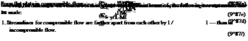
Equation (9.79) is valid only for streamlines away from the body. Since the Prandtl-Glauert transformation is based on small perturbation theory, the error increases with increasing thickness of the body. In addition to this, some error is introduced by the above contradiction [see Equation (9.85)].

Equation (9.86) shows that the streamlines around a body in a compressible flow are more separated than those around a body in incompressible flow by an amount given by 1/ 1 — M^,. In other words,

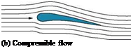by the existence of body in the flow field, the streamlines are more displaced in a compressible flow than in an incompressible flow, as shown in Figure 9.8, that is the disturbances introduced by an object are larger in compressible flow than in incompressible flow and they increase with the rise in Mach number. This is so because in compressible flow there is density decrease as the flow passes over the body due to acceleration, whereas in incompressible flow there is no change in density at all. That is to say, across the body there is a drop in density, and hence by streamtube area-velocity relation (Section 2.4, Reference 1), the streamtube area increases as the density decreases. At Mx = 1, this disturbance becomes infinitely large and this treatment is no longer valid.

(a) Incompressible flow

Figure 9.8 Aerofoil in an uniform flow.

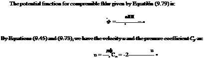Using Equation (9.87a), the perturbation velocity and the pressure coefficient may be expressed as follows:

дф _ 1 дф|пс

dx V/1—dxinc’

Therefore:

u inc

u = —, •

v/1-ML

Since the lift coefficient CL and pitching moment coefficient CM are integrals of CP, they can be expressed following Equation (9.87b) as:

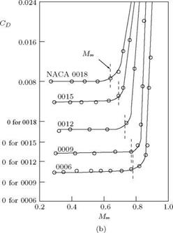
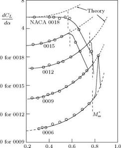
Variation of (a) lift-curve slope and (b) drag coefficient with Mach number (o-measured).

2. The ratio between aerodynamic coefficients in compressible and incompressible flows is also

1Л/1 – .

From Equations (9.87c) and (9.87f), we infer that the locations of aerodynamic center and center of pressure do not change with the freestream Mach number Mx, as they are ratios between CM and CL.

The theoretical lift-curve slope and drag coefficient from the Prandtl-Glauert rule and the measured CL and CD versus Mach number for symmetrical NACA-profiles of different thickness are shown in Figure 9.9.

From this figure it is seen that the thinner the aerofoil the better is the accuracy of the P-G rule. For 6% aerofoil there is good agreement up to MOT = 0.8; for 12% aerofoil also, the agreement is good up to Mx = 0.8; thus 12% may be taken as the limit of applicability of the Prandtl-Glauert (P-G) rule. For 15% aerofoil, there is good agreement up to MOT = 0.6. But above Mach 0.6, there is no more agreement. However, for supersonic aircraft the profiles used are very thin; so from a practical point of view, the P-G rule is very good even with the contradicting assumptions involved.

Beyond a certain Mach number, there is decrease in lift. This can be explained by Figure 9.9(b). There is sudden increase in drag when the local speed increases beyond sonic speed. This is because at sonic point on the profile, there is a X —shock which gives rise to separation of boundary layer, as shown in Figure 9.10.

The freestream Mach number which gives sonic velocity somewhere on the boundary is called critical Mach number M^. The critical Mach number decreases with increasing thickness ratio of profile. The P-G rule is valid only up to about M^.

Moo