Spatial Resolution Requirements

In designing a computational grid, the first question one faces is “what size mesh to use.” This question cannot be answered until one has some idea of the flow and acoustic fields as well as the size of acoustic sources involved. Even if they are known, it is still not straightforward to decide what size mesh to use. For instance, if the flow contains a free shear layer of vorticity thickness, 8a, what mesh size to use is not completely obvious unless one has previous experience. The purpose of this section is to develop quantitative criteria to assist in selecting a proper mesh size for aeroacoustics computation.

15.2.1 Free Shear Flows

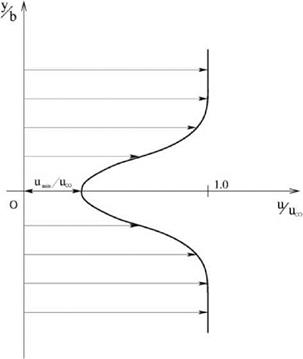
As an illustration of how one may formulate a mesh size selection procedure, consider the problem of computing a low Mach number two-dimensional wake flow of half­width b. According to the book by White (1991), the velocity deficit, U, of such a wake flow, whether it is laminar or turbulent, has the profile of a Gaussian function, i. e.,

The velocity profile is shown in Figure 15.1.

For computational purposes, the mesh size is to be assigned so as to be capable of resolving the Gaussian function part of the flow. Now, note that the Fourier transform of a Gaussian function is a Gaussian function, i. e.,

where a is the wave number. It is easy to show that the area under the wave number spectrum of Eq. (15.2) is unity, i. e.,

TO

j S(a)da = 1.

-TO

Figure 15.1. Velocity profile of a two­dimensional turbulent wake.

The fraction of the wave number spectrum up to a wave number k, denoted by F(kb), is

k

F(kb) = 2 j S(a)da = erf
0

where erf [ ] is the error function. If the mesh size is chosen to resolve the wake flow up to a wake number k, then the fractional error, E(kb), is equal to

A plot of E(kb) is shown in Figure 15.2.

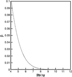
Suppose the 7-point stencil DRP scheme is chosen to do the computation. This scheme is acceptable if the mesh size Ay is chosen so that kAy < 0.95 (see Chapter 2). Now consider that a fractional error в (в << 1.0) is acceptable for the computation; then, by using the 7-point stencil DRP scheme, the mesh size would be given by equating E(kb) to в with k = (0.95/Ay). This gives

of 2b/Ay. Now, for an assigned value of в, there is a corresponding value of 2b/Ay, say a. Thus, the maximum mesh size allowed is

2b

(АУ ^maximum = — • (15.6)

a

By following this procedure, the maximum mesh size for a given acceptable error for other shear flows can be readily established. For the cases of a two-dimensional

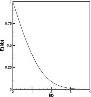Figure 15.3. Spatial resolution curve for two-dimensional wake flow.

Figure 15.4. Velocity profile of a two­dimensional turbulent mixing layer.

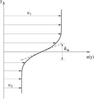mixing layer, a two-dimensional turbulent jet, a laminar boundary layer, and a tur­bulent boundary layer, the spatial resolution curves are provided in the following sections.