Laminar Boundary Layer

Now, boundary layer flows are quite different from free shear layers. Unlike free shear flows, boundary layer flows occupy only a half-infinite space. Furthermore, boundary layers have a substantially different mean velocity profile. Because of these differences, it is necessary to modify slightly the mesh size selection procedure. For example, consider a low-speed flat-plate boundary layer of thickness 5 (99 percent) in a free stream flow of velocity uC. The mean flow has a well-known similarity

Figure 15.8. Velocity profile of a laminar boundary layer and its reflection.

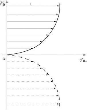profile. It is given by the Blasius solution (see Figure 15.8). In standard notation (White, 1991), it is as follows:

— = f (n), n = ^ (f (3-5) = 0-99).

йж S

To facilitate the computation of the wave number spectrum, it is recommended to regard the problem as one to compute the velocity deficit as follows:

— (Щ = [1 – f (Ini)] (15.10)

instead of the mean velocity. Note: Eq. (15.10) extends the velocity deficit to the full range —ж < y < ж by a simple reflection.

Now, the Fourier transform of —, denoted by S, is

ж ж

S(ff) = 2П f — (^)e—iaydy = 7- j [1 — f (ini)] Є3-5ndn. (15.11)

— ж —ж

It is easy to show that the area under the wave number spectrum is unity. Therefore, the normalized wave number spectrum is given by Eq. (15.11). Thus, the fractional error by using the 7-point stencil DRP scheme is

0.95

e=1—2 К35)da