Mesh Design: Body-Fitted Grid

The importance of having a well-designed grid in a numerical simulation cannot be overemphasized. For problems involving solid surfaces, a body-fitted grid is most desirable. Computation on such a grid has the advantage that the wall boundary conditions can be enforced with relative ease and accuracy. With body-fitted grid, one set of grid lines will be parallel to the solid surface. This is ideal for computing the boundary layer adjacent to the wall. Developing a body-fitted grid is not straight­forward. Grid generation is, by itself, a topic that has been extensively researched. The subject matter is treated in specialized books and advanced texts. It is beyond the scope of this book to treat grid generation other than providing an example to illustrate some aspects of the basic ideas.

15.3.1 Conformal Transformation

Consider the problem of computing the flow around a two-dimensional airfoil. A simple way to generate a body-fitted grid for the airfoil is to use the method of conformal mapping.

Figure 15.15. Mapping of an airfoil into a slit by conformal mapping. Open cir­cles are sources points on the camber line. Black circles are enforcement points.

The method consists of two essential steps as schematically illustrated in Figures 15.15, 15.16, and 15.17. The first step is a mapping of the airfoil in the physical x – y plane into a slit in the w or the f – n plane. This is accomplished by conformal transformation using a multitude of point sources or doublets distributed along the camber line of the airfoil as shown in Figure 15.15. If point sources are used, the appropriate form of the conformal transformation is

w = z + £ Qj log Z—j + in, (15.17)

j=1 z z0

where w = f + in is the complex coordinates of a point in the mapped plane, z = x + iy is a point in the physical plane, Qj, Zj (j = 1,2,…, N) are the source strengths and locations, and П is just a constant. The inclusion of П in the mapping function is important. Its inclusion makes it possible to map the airfoil onto a slit on the real axis of the w plane (see Figure 15.16). z0 is the location of a reference source. A good location to place z0 is in the middle of the camber line, such that all the lines joining zj to z0 lie within the airfoil. In this way, the branch cuts associated with the log functions of Eq. (15.17) would not present a problem in the computation.

In implementing the mapping, the coordinates Zj (j = 1,2,3,…, N) of the source points are first assigned. A useful rule in assigning the source locations is that the distance |Zj – Zj_x| should be in some way proportional to the local thickness of the airfoil. That is to say, the sources should be closer together at where the airfoil is thin. Now the source strengths Qj (j = 1,2,…, N) are to be chosen to accomplish the mapping. For this purpose, a set of points, zk (k = 1,2,…, M), well distributed around the surface of the airfoil is chosen to enforce the mapping (see Figure 15.15). zk are the enforcement points, and M should be much larger than N. On imposing the conditions that the surface of the airfoil be mapped onto a slit on the real axis of

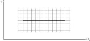Figure 15.16. Complex w plane. The slit is the airfoil.

the w plane, Eq. (15.17) leads to the following system of linear equations for Qj and ft:

This system of equations may be written in a matrix form (real variable) as follows:

Ax = b,

where x is a column vector of length (2N + 1). The elements of x are

X2j—1 = Re (Qj), X2j = Im(Qj), j = 1, 2,…, N

X2N+1 = ft.

A is a M x (2N + 1) matrix. The elements of A are

Г zi — zi"

ai,2 j + iai,2 j—1 = log

zi z0

ai,2N+1 = 1’i = 1, 2, . . . , M; j = 1, 2, 3, . . . , N.

b is a column vector of length M. The elements of b are

bk = —yk, k = 1, 2, 3,…, M.

With M > 2N + 1 Eq. (15.19) is an overdetermined system. A least squares solution may be obtained by first premultiplying Eq. (15.19) by the transpose of A. This leads to the normal equation,

ATAx = ATb, (15.20)

which can be easily solved by any standard matrix solver.

If a point dipole distribution is used to map an airfoil into a slit instead of point sources, the mapping function would be

The mapping constants zj, Aj(j = 1, 2,…) and C are determined in the same way as those for point sources.

The second step in developing a body-fitted grid to the airfoil is to take the midpoint of the slit in the f – n plane as the center of an elliptic coordinate system. The two end points of the slit are the singular points of the conformal transformation. They are given by

dw = 0.

dz

Let the width of the slit be a and f be the x coordinate measured from the midpoint of the slit. The elliptic coordinates (д, в) are related to (f, n) by

f = 2 cosh д cos в, n = a sinh д sin в. (15.23)

The elliptic coordinate system is shown in Figure 15.17. The elliptic coordinate system is orthogonal. The curve д = 0 is the surface of the airfoil in the physical plane. If the computation is for a flow past the airfoil, then the boundary layer lies in the region д < A in the д – в plane. The wake is in the region – A1 < в < Д2, where A, A1; and Д2 are small quantities for a flow fromleft to right. In a simulation, these are the regions where very fine meshes are needed.