. Turbulent Boundary Layer

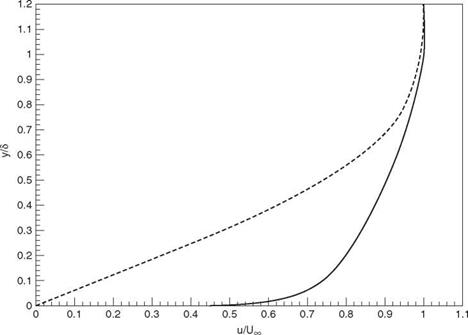
The velocity profile of a turbulent boundary layer over a flat plate consists of three distinct layers. They are the viscous sublayer, the log layer, and the outer wake layer. Figure 15.10 shows the velocity profile of a turbulent boundary layer at low Mach number. The velocity profile is constructed by using the law of the wake profile for the outer layer and Spalding’s formula for the inner layer. The viscous sublayer is very thin and has a very large velocity gradient. It accounts for less than 1 percent of the boundary layer thickness. The log layer lies on top of the viscous layer. It makes up about 20 percent of the boundary layer thickness. The log layer may be regarded as a transition layer. The top layer is the wake flow. It constitutes the bulk (~80 percent) of the boundary layer. In this layer, the velocity gradient is the mildest. Because of the large variation of mean flow velocity gradient across the boundary layer, it is not feasible to use a single size mesh for its computation. The mesh size needed to resolve each of the three layers will be considered separately below.

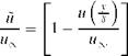
Let the velocity profile of a low-speed flat-plate turbulent boundary layer be u(y/5), where 5 is the boundary layer thickness. As in the case of laminar boundary layer, the velocity deficit U (see Figure 15.11a) may be written in the following form:

Figure 15.10. Velocity profile of a turbulent boundary over a flat plate (dark curve) and that of a laminar boundary layer (dotted curve).

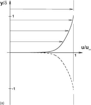Figure 15.11a. Profile of velocity deficit й/и^ of a low-speed turbulent boundary layer.

Figure 15.11b. Profile of velocity deficit u-20%/ure of a low-speed turbulent boundary layer.

The Fourier transform of the velocity deficit, extended to the full range – re < y

< re, is

A change of variable leads to

It is easy to show that the area of the wave number spectrum is unity. Suppose the 7-point stencil DRP scheme is used for computation, then the fractional error в for using a computational mesh size Ay is

°-95( y)

в = 1 — 2 ‘S(Z)dZ. (15.15)

0

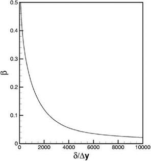
The numerical solution of Eq. (15.15) is given in Figure 15.12. By means of this figure, it is a simple matter to make a quantitative estimate of the maximum mesh size Ay permissible for a prescribed fractional error в. In this way, the mesh size required to compute the viscous sublayer is found.

To find the mesh size needed to resolve the log layer, one may use essentially the same procedure as before. Consider a turbulent boundary layer with the bottom 2 percent removed, that is, the viscous sublayer is taken out from consideration. Let the new mean velocity profile be u—2<% (|). Now, apply this analysis to u -2% (S), the new velocity deficit with a symmetric extension to the negative y plane is

Figure 15.12. Spatial resolution curve for the viscous sublayer of a turbulent bound­ary layer.

The mesh size requirement for computing velocity deficit profile Eq. (15.16) by the 7-point stencil DRP scheme may be determined in the same way as velocity deficit profile Eq. (15.13). Figure 15.13 shows the mesh size resolution curve, в versus 5 /Ay, for computing the log layer of a turbulent boundary layer. This procedure may be applied to the wake layer as well. This is done by deleting the lower 20 percent of the boundary layer velocity profile as shown in Figure 15.11b. On proceeding as

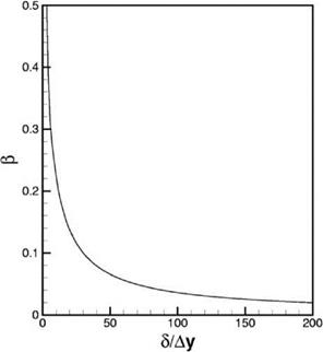Figure 15.13. Spatial resolution curve for the log layer of a turbulent boundary layer.

Figure 15.14. Spatial resolution curve for the wake layer of a turbulent bound­ary layer.

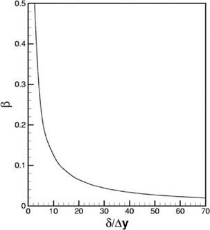above, it is straightforward to derive the mesh resolution curve for computing the outer wake layer. Figure 15.14 is the в versus S/Ay curve.

On comparing Figures 15.12,15.13, and 15.14, it is evident that there are orders of magnitude of difference in the mesh size requirement in computing the three layers of a turbulent boundary layer. This is probably not too surprising. In a realistic computation, a multisize mesh is absolutely necessary. Such a computation can be handled by the multi-size-mesh multi-time-step method discussed in Chapter 12.