The agility factor

One of the most common causes of dispersion in pilot HQRs stems from poor or im­precise definition of the performance requirements in an MTE, leading to variations in interpretation and hence perception of achieved task performance and associated workload. We have already illustrated this with the controlled experiment data from the AFS slalom and sidestep MTEs. In operational situations, this translates into the variability and uncertainty of task drivers, commonly expressed in terms of precision, but the temporal demands are equally important. The effects of task time constraints on perceived handling have been well documented (Refs 7.20-7.24) and represent one of the most important external factors that impact pilot workload. Flight results gathered on Puma and Lynx test aircraft at DRA (Refs 7.20, 7.23, 7.24) showed that a critical parameter was the ratio of the task performance achieved to the maximum available from the aircraft; this ratio gives an indirect measure of the spare capacity or performance margin and was consequently named the agility factor. The notion developed that if a pilot could use the full performance safely, while achieving desired task precision requirements, then the aircraft could be described as agile. If not, then no matter how much performance margin was built into the helicopter, it could not be described as agile. The DRA agility trials were conducted with Lynx and Puma operating at light weights to simulate the higher levels of performance margin ex­pected to be readily available, even at mission gross weights, in future types (e. g., up to 20-30% hover thrust margin). A convenient method of computing the agility factor was developed as the ratio of ideal task time to actual task time. The task was deemed to commence at the first pilot control input and to complete when the aircraft motion decayed to within prescribed limits (e. g., position within a prescribed cube, rates <5°/s) for repositioning tasks, or when the accuracy/time requirements were met for tracking or pursuit tasks. The ideal task time is calculated by assuming that the maximum acceleration is achieved instantaneously, in much the same way that some aircraft models work in combat games. So, for example, in a sidestep repositioning manoeuvre, the ideal task time is derived with the assumption that the maximum transla­tional acceleration (hence aircraft roll angle) is achieved instantaneously and sustained for half the manoeuvre, when it is reversed and sustained until the velocity is again zero.

The ideal task time is then simply given by

Ti = J(4S/amax) (7.3)

where S is the sidestep length and amax is the maximum translational acceleration. With a 15% hover thrust margin, the corresponding maximum bank angle is about 30°, with amax equal to 0.58 g. For a 100-ft sidestep, T then equals 4.6 s. Factors that increase the achieved task time, beyond the ideal, include

(1) delays in achieving the maximum acceleration (e. g., due to low roll attitude bandwidth/control power);

(2) pilot reluctance to use the maximum performance (e. g., no carefree handling capability, fear of hitting ground);

(3) inability to sustain the maximum acceleration due to drag effects and sideways velocity limits;

(4) pilot errors of judgement leading to terminal repositioning problems (e. g., caused by poor task cues, strong cross-coupling).

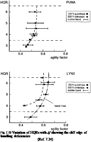
To establish the kinds of agility factors that could be achieved in flight test, pilots were required to fly the Lynx and Puma with various levels of aggressiveness or ma­noeuvre ‘attack’, defined by the maximum attitude angles used and rate of control application. For the low speed, repositioning sidestep and quickhop MTEs, data were gathered at roll and pitch angles of 10°, 20° and 30° corresponding to low, mod­erate and high levels of attack, respectively. Figure 7.19 illustrates the variation of HQRs with agility factor for the two aircraft (Ref. 7.24). The higher agility factors achieved with Lynx are principally attributed to the hingeless rotor system and faster engine/governor response. Even so, maximum values of only 0.6-0.7 were recorded compared with 0.5-0.6 for the Puma. For both aircraft, the highest agility factors were achieved at marginal Level 2/3 handling. In these conditions, the pilot is either working with little or no spare capacity, or not able to achieve the flight path pre­cision requirements. According to Fig. 7.19, the situation rapidly deteriorates from Level 1 to Level 3 as the pilot attempts to exploit the full performance, emphasizing the ‘cliff edge’ nature of the effects of handling deficiencies. The Lynx and Puma are typical of current operational types with low authority stability and control aug­mentation. While they may be adequate for their current roles, flying qualities defi­ciencies emerge when simulating the higher performance required in future combat helicopters.

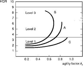
The different possibilities are illustrated in Fig. 7.20. All three configurations are assumed to have the same performance margin and hence ideal task time. Configuration

A can achieve the task performance requirements at high agility factors but only at the expense of maximum pilot effort (poor Level 2 HQRs); the aircraft cannot be described as agile. Configuration B cannot achieve the task performance when the pilot increases his or her attack and Level 3 ratings are returned; in addition, the attempts to improve task performance by increasing manoeuvre attack have led to a decrease in agility factor, hence a waste of performance. This situation can arise when an aircraft is PIO prone, is difficult to re-trim or when control or airframe limits are easily exceeded in the transient response. Configuration B is certainly not agile and the proverb ‘more haste, less speed’ sums the situation up. With configuration C, the pilot is able to exploit the full performance at low workload. The pilot has spare capacity for situation awareness and being prepared for the unexpected. Configuration C can be described as truly agile. The inclusion of such attributes as safeness and poise within the concept of agility emphasizes its nature as a flying quality and suggests a correspondence with the quality levels. These conceptual findings are significant because the flying qualities boundaries, which separate different quality levels, now become boundaries of available agility. Although good flying qualities are sometimes thought to be merely ‘nice to have’, with this interpretation they can actually delineate a vehicle’s achievable performance. This lends a much greater urgency to defining where those boundaries should be. Put simply, if high performance is dangerous to use, then most pilots will avoid using it.

In agility factor experiments the definition of the level of manoeuvre attack needs to be related to the key manoeuvre parameter, e. g., aircraft speed, attitude, turn rate or target motion. By increasing attack in an experiment, we are trying to reduce the time constant of the task, or increasing the task bandwidth. It is adequate to define three levels – low, moderate and high, the lower corresponding to normal manoeuvring, the upper to emergency manoeuvres.

There are also potential misuses of the agility factor when comparing aircraft. The primary use of the A f is in measuring the characteristics of a particular aircraft performing different MTEs with different performance requirements. However, Af also compares different aircraft flying the same MTE. Clearly, a low-performance aircraft will take longer to complete a task than one with high performance, all else being equal. The normalizing ideal time will therefore be greater for the lower than the higher performer, and if the agility factors are compared, this will bias in favour of the poor performer. Also, the ratio of time in the steady state to time in the transients may well be higher for the low performer. To ensure that such potential anomalies are not encountered, when comparing aircraft using the agility factor it is important to use the same normalizing factor – defined by the ideal time computed from a performance requirement.