Our heavyweight helicopter equal in the world does not have
In Rostov started production of the most load-lifting rotary-wing car The Russian holding «Helicopt[...]

Everything about aircrafts and helicopters. News and events in aviation worldwide. Civil, transportation, military helicopters and airplanes.

Everything about aircrafts and helicopters. News and events in aviation worldwide. Civil, transportation, military helicopters and airplanes.

Everything about aircrafts and helicopters. News and events in aviation worldwide. Civil, transportation, military helicopters and airplanes.

Everything about aircrafts and helicopters. News and events in aviation worldwide. Civil, transportation, military helicopters and airplanes.


A well-designed grid is crucial to an accurate numerical simulation. For flow past an airfoil, accurate resolution of the boundary layer and wake flow is very important. To be able to do so, the use of a body-fitted grid is most advantageous.
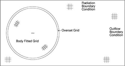
The problem at hand is a multiscales problem. The smallest length scale of the problem that needs to be resolved is in the viscous boundary layer and in the wake. In this work, a multisize mesh is used in the time marching computation. Figure 15.24 shows the overall computational domain. It extends to a distance of 10 chordlengths in front of the leading edge of the airfoil and 30 chords downstream. The lateral dimension is 20 chords. The reason for choosing such a large computational domain is to provide sufficient distance for the wake flow and vortices to develop fully and to decay sufficiently before exiting the outflow boundary. A body-fitted elliptic coordinate system (p,, в) and mesh, as discussed in the Section 15.3, is used around the
|
Figure 15.24. Computational domain in physical space for uniform flow past an airfoil. |
airfoil. This region extends to a radius of 8 chords (for large д, the elliptic coordinate system evolves into a polar coordinate system). Outside this nearly circular region, a Cartesian grid is used. This is illustrated in Figure 15.24. An overset grid region is created to encircle the body-fitted mesh. It is used to transfer computational information between the Cartesian grid and the body-fitted grid. The overset grid method of Chapter 13 is implemented here.
The boundary layer flow adjacent to the airfoil and the wake flow are believed to be responsible for the generation of airfoil tones. It is, therefore, important to provide sufficient spatial resolution in computing the flow in these thin shear layers. For this reason, in the grid design, the smallest size meshes are assigned to these regions. The grid layout in the д – в plane (the computational domain for the elliptic coordinate region) is as shown in Figure 15.25. In this figure, the range of в is from – n to n with periodic boundary conditions imposed on the left and right boundaries. The airfoil surface is on the line д = 0. This computational domain is divided into seventeen subdomains, symmetric about the line в = 0. The subdomains are labeled by a capital letter “A,” “B,” “C,” etc. In the physical plane, these subdomains are shown in Figures 15.26 and 15.27. Subdomains “B” and “C” contain the boundary layer. Subdomains “A” and “D” contain the near wake. Subdomains “F,” “H,” and “M” contain the intermediate wake. The far wake is in subdomain “N.” Subdomain “N” extends to the edge of the Cartesian grid region. Table 15.1 provides the mesh size assigned to each of the computational subdomains with Дв0 = 0.00218 and Дд0 = 0.0015. The mesh size of the Cartesian grid is uniform with Дх = Ду = 0.053.