15.4.2.2 Acoustics

In all the simulations that have been performed for Airfoils #1, #2, and #3 (see Table 15.2). only a single tone is detected. Figure 15.37 shows a typical airfoil trailing

edge noise spectrum. This is the noise spectrum of Airfoil #1 at a Reynolds number of 4 x 105. The measurement point is at (1.08, 0.5). Since there is only one single tone per computer simulation, it makes the finding the same as Nash et al. (1999).

Figure 15.38 shows the computed tone frequencies versus flow velocities for Airfoil #1 according to the results of our numerical simulations. This airfoil has a 0.5 percent truncation. It is nearly a sharp trailing edge airfoil. As shown in this figure, all the data points lie practically on a straight line parallel to the Paterson formula (the full line). The difference between the simulation results and the Paterson formula

is very small. On the basis of what is shown in Figure 15.38, it is believed that the simulations, for all intents and purposes, reproduce the empirical Paterson formula. The good agreement with the Paterson formula not only is a proof of the validity of the simulations, but also is an assurance that numerical simulations do contain the essential physics of airfoil tone generation.

Figure 15.39 shows the variations of the Strouhal numbers of the computed tones with Reynolds number for the three airfoils under consideration. The data for each airfoil lies approximately on a straight line. The straight lines are parallel to each

other and to the Paterson formula (shown as the full line in Figure 15.39). All the four lines in Figure 15.39 fit a single formula as follows:

fC 1

Ц – = KRe2, (15.58)

where K is a constant. Eq. (15.58) may also be written in the form similar to the Paterson formula, i. e.,

3

U 2

f = K——– 1. (15.59)

(Cu)2

The values of constant K for each airfoil have been determined by best fit to the simulation data. They are given in Table 15.3.

Based on the computed results shown in Figure 15.39, the effect of trailing edge thickness at a given Reynolds number is to lower the tone frequency, that is, the thicker the blunt trailing edge the lower is the tone frequency. This dependence turns out to be similar to that of vortex shedding tones, such as that emitted by a long circular cylinder in a uniform flow. For the long cylinder vortex shedding problem, the tone Strouhal number is approximately equal to 0.2, i. e.,

fD

— & 0.2 (D is the diameter). (15.60)

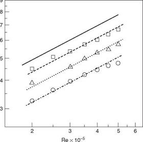Figure 15.39. Dependence of tone Strouhal number on Reynolds number

for Airfoils #1, #2, and #3.—– , Airfoil

#1,…………. Airfoil #2;——– , Airfoil #3;

—– , Paterson formula.

Therefore, the thicker the blunt object or trailing edge, the lower the tone frequency is. However, note that the physics and tone generation mechanisms are quite different.