Our heavyweight helicopter equal in the world does not have
In Rostov started production of the most load-lifting rotary-wing car The Russian holding «Helicopt[...]

Everything about aircrafts and helicopters. News and events in aviation worldwide. Civil, transportation, military helicopters and airplanes.

Everything about aircrafts and helicopters. News and events in aviation worldwide. Civil, transportation, military helicopters and airplanes.

Everything about aircrafts and helicopters. News and events in aviation worldwide. Civil, transportation, military helicopters and airplanes.

Everything about aircrafts and helicopters. News and events in aviation worldwide. Civil, transportation, military helicopters and airplanes.


It was mentioned at the beginning of this chapter that, at present, there are two approaches to LES. One approach uses a subgrid scale model. The idea is to cut off and not to compute the very high wave number part of the turbulence spectrum. To account for the effect of the cutoff spectrum on the larger-scale turbulent motion, a model of the stress-strain rate relation is used. It turns out that a subgrid scale model based on a stress-strain rate relation does not simulate the effect very well. Such a model effectively provides only damping terms to the fluid motion, especially the high wave number components. This prevents the accumulation of small-scale turbulence energy due to the cascade process (energy continues to cascade to the shorter and shorter scales or higher and higher wave number components). The alternative approach is to use numerical damping to perform the same task. A natural way, in the later case, is to use artificial selective damping. For this purpose, the a = 0.3n damping curve of Section 7.2 may be used. There is no sharp cutoff for this damping curve. A reasonable choice is to take the cutoff wave number to be approximately at a Ax = 1.6.
Instead of using artificial selective damping, one may use filtering. Filtering is a way to eliminate high wave number components with minimal effect on the long waves. A one-dimensional numerical filter may be constructed as follows.
Let f be the value of a dynamical variable at the I th mesh point. Consider a 7-point stencil filter. A filter should be symmetric to avoid any chance of amplifying the filtered value. Suppose f is the filtered value. The filtered value is related to the original values on the computational stencil by the following relation (assuming a linear filter is used).
fl = A( ft+3 + fl-3 ) + B( fl+2 + fl-2) + C( ft+1 + fl-1) + Dfl. (15.66)
The Fourier transform of Eq. (15.66) is
f = [2A cos(3aAx) + 2B cos(2aAx) + 2Ccos(aAx) + D] f = F(aAx) f. (15.67) On inverting the Fourier transform, the filtered function becomes
f(x) = f F(aAx)feiaxda. (15.68)
It is clear that the function F(a Ax) in Eq. (15.68) regulates the band of wave numbers that contributes to the filtered value of the original function. For this reason, F (a Ax) is referred to as the filter function.
1.0
Figure 15.49. An ideal filter with a cutoff : :r v,
at a Ax = pn.
![]()
Ideally, if all the wave numbers larger than a Ax > pn associated with a turbulence field are to be discarded or ignored, then the desirable filter function would be
|
|||
|
|
||
This ideal filter function is shown in Figure 15.49. When a finite size stencil is used, it is not possible to construct an ideal filter function. Thus, the objective is to make the filter as close to the ideal filter as possible.
For a 7-point stencil filter function, there are four free parameters. These parameters will now be determined by requiring the following conditions be satisfied.
![]() F (0) = 1.0
F (0) = 1.0
![]() з 2f
з 2f
d(aAx)2 aAx=0 3 4F
d(aAx)4 aAx=0
F (n) = 0
It is easy to show that the values of the coefficients that satisfy these constraints are as follows:
A = 64^ B = 32’ C = 14- D = 11. (15.70)
Thus the filtering formula is
fl = 64 (ft+3 + fl-3 ) – 32 (ft+2 + fl-2) + 15 (fl+1 + fl-1) + Ц ft. (15.71)
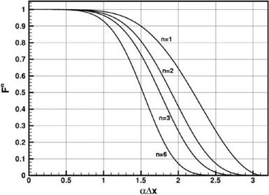
The filter function F (a Ax) is shown as the n = 1 curve in Figure 15.50. This figure does not look like the ideal filter function. To make the filter function resembling more of the ideal filter, one may perform repeated filtering. It is straightforward to show if the filtering process is performed n number of times, the filtered function becomes
TO
f(x) = F (aAx) h. V-da.
— TO
|
Figure 15.50. Profile of several 7-point stencil filter functions in wave number space. |
That is, repeated filtering amounts to using a high power of the original filter function. Figure 15.50 shows a plot of F2 (a Ax), F3 (a Ax), F6(a Ax), i. e., n = 2, 3, 6. It is clear that the filter function to a high power has a better resemblance to the ideal filter. However, it is not advisable to perform many filtering operations in one time step, because it will degrade the solution in the long wave range. If n = 3 filter is used, the approximate cutoff wave number, taken to be F3 (acutoff Ax) = 0.5, is given
by acutoffAx ^ 1.8.